Sugar-rich foods exacerbate antibiotic-induced microbiome disruption – Nature

Patients

In this cohort study of adult allo-HCT recipients at Memorial Sloan Kettering Cancer Center in New York between 2017 and 2022, eligible participants had been admitted for Allo-HCT. Three times weekly, patients who had been recently admitted for allo-HCT were invited to participate in dietary-intake collection. Neutrophil engraftment was defined as the first of 3 days of neutrophil count ≥500 per μl. Five patients died without achieving engraftment and were excluded from the analysis of median time to engraftment. No patients were lost to follow-up. For mortality analysis, one patient died before landmark day 12 and was excluded from that analysis. The latest follow-up/data collection date was in April 2023.

Nutrition data collection and annotation

The hospital kitchen commercial computer system (Computrition) was configured to provide a printout that accompanied each meal tray to the bedside on which patients were asked to indicate, immediately after each meal, whether they consumed 0, 25%, 50%, 75% or 100% of each item they ordered for that meal. These instruments were collected by a dietician or other research team members three times weekly, during which missing entries were completed at the bedside along with encouragement to sustain motivation with the project. Consumption data were entered into the kitchen software, which was linked to the recipe and mass of each item. Data were manually vetted by a research dietitian for quality control (for example, grossly implausible kcal values resulting from sporadic typographic errors in the hospital kitchen records). Habitual dietary patterns before admission were not surveyed; the analysis was focused on inpatient dietary intake. Per-patient intercept terms were included in the Bayesian model (see below), which may capture interpatient variability in unmeasured parameters such as patient-specific pretransplant dietary habits.

An eight-digit food code was assigned to each unique food item according to the classification of the FNDDS⁴⁶. The numeric codes are structures such that subsequent numeral positions differentiate foods within larger groups. For example, in the food code 14109010 for Swiss cheese, the first digit, 1, denotes milk and milk products; the second digit, 4, denotes cheeses; and each subsequent digit conveys progressively higher resolution classifications of foods. We removed the water content from the food total weight before analysis. To compute the dehydrated weight of consumed foods, we subtracted the water content, derived from FNDDS water fractions, from the total food weight. However, for EN, which is administered as a liquid and lacks a standardized total weight in grams, we used an additive approach. The dehydrated weight for these enteral formulations was calculated by summing the total gram weight of their protein, fat and carbohydrate components. This approach allows a more accurate comparison of nutrient intake across individuals and different food types, as it eliminates the variability introduced by water content. Therefore, when we refer to each 100 g increase in sweets, we are referring to 100 g of the dehydrated weight of foods within the ‘sweets’ category. This ensures that we are comparing the actual nutrient content, including sugar, rather than the total weight or volume of the food consumed. The analysed dataset therefore listed the dehydrated weight in grams of FNDDS food items consumed in each meal on each day of hospitalization.

Foodtree construction

A food tree was constructed with the 622 unique FNDDS items consumed by the patients in this cohort, as done previously⁷ (https://github.com/knights-lab/Food_Tree). The tree spans nine broad FNDDS food groups, namely, grain products (abbreviated here as grains); vegetables; meat, poultry, fish and mixtures (abbreviated here at meats); milk and milk products (abbreviated here as milk); sugars, sweets and beverages (abbreviated here as sweets); fruits; dry beans, peas, other legumes, nuts and seeds (abbreviated here as legumes); fats, oils and salad dressings (abbreviated here as fats); and eggs. In some cases, food items not explicitly classified in FNDDS contained ingredients from multiple categories (such as milk-based mango smoothie). We addressed this by manually categorizing foods on the basis of which FNDDS food description they fit best to. For example, milk-based mango smoothie, despite having mango in it, fits the description of ‘11553110 fruit smoothie, with whole fruit and dairy’; it was therefore classified in the ‘milk and milk products’ group.

Dietary data analysis: TaxUMAP and diet α-diversity

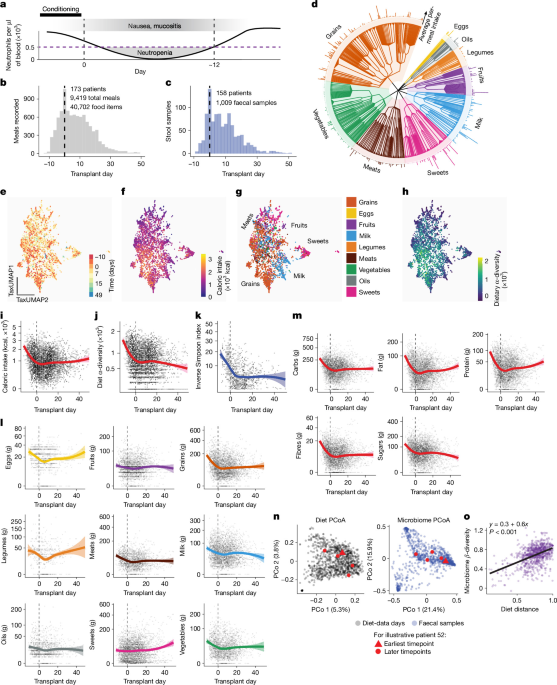
The hierarchical organization of the FNDDS vocabulary facilitated application of α-diversities to diet data using Faith’s phylogenetic distance⁴⁷, which was implemented in Qiime2 (qiime2-2021.11)⁴⁸ using the qiime diversity alpha-phylogenetic function with the faith_pd metric. The food tree taxonomy was used, as well as the dehydrated weight consumption of the food item represented by food code per patient per day. The TaxUMAP method⁴ was used to visualize compositional similarities between the patients’ daily meals, similar to β-diversity. The fraction of each consumed food represented by a food code per patient per day was used to calculate the food tree taxonomy. Trends in microbiome and nutrition dynamics over time (Fig. 1i–k) were analysed by GEEs using the geeglm function in geepack (v.1.3.9) in R.

Human faecal microbiome analysis

Faecal sample inclusion criteria and flow through the study are detailed in Extended Data Fig. 1a. Samples were transported from the inpatient transplant unit to the laboratory through a pneumatic tube system at room temperature, promptly refrigerated and then aliquoted and frozen at −80 °C within 1 business day. Microbiome profiling by 16S rRNA sequencing was performed in the MSK Molecular Microbiology Facility as described⁴⁹. In brief, bacterial cell walls were disrupted, and nucleic acids isolated using silica bead-beating and phenol–chloroform extraction, and the V4–V5 variable region of the 16S rRNA gene was amplified. Amplicons were purified using either the Qiagen PCR Purification Kit (Qiagen) or AMPure magnetic beads (Beckman Coulter) and quantified using the Tapestation instrument (Agilent). No enrichment of microbial DNA was performed. DNA was pooled to equal final concentrations for each sample and then sequenced on the Illumina platform. Of the 1,009 human faecal samples in this study, 42 were sequenced more than once. The median Bray–Curtis distance between distinct microbiome profiles generated from these same samples was 0.01, which was substantially smaller than the distance between samples from the same patients collected on different days (median value, 0.54; P < 0.0001) and also smaller than the distance between samples from different patients (median value, 0.89; P < 0.0001). This suggests that much more variation in composition is explained by biological differences than by technical sequencing variation. The median read count was 132,978 and the range was from 1,196 to 8,698,524. The 16S sequencing data were analysed using the R package DADA2 (v.1.16.0) pipeline with the default parameters except for maxEE=2 and truncQ=2 in the filterandtrim() function⁵⁰, 16S FASTQ files were capped at 10⁵ reads per sample. ASVs were annotated according to NCBI 16S database using BLAST⁵¹. Microbiome α-diversity was evaluated using the inverse Simpson index—a summary statistic of both the richness and evenness of the bacterial community. Taxa abundances were summarized at the genus level.

Relationships between microbiome α-diversity and clinical factors such as conditioning intensity, exposures to antibiotics, sweets and parenteral nutrition were analysed mainly through Bayesian models that accounted for repeated sampling, time relative to transplantation and other patient-level variables (see the ‘Bayesian multilevel model’ section below). To facilitate visualization of relationships in the unadjusted raw dataset, α-diversity values in various sample subsets are plotted as beeswarm plots in Extended Data Fig. 1f.

To address taxonomic heterogeneity within the Enterococcus genus and the pattern that E. faecium is the most commonly dominating species in this dataset (Extended Data Fig. 7d), we constructed a hybrid taxonomic feature table for the β-diversity analysis in Extended Data Fig. 3. In this taxonomic feature table, the Enterococcus genus was partitioned into two distinct features: (1) Enterococcus ASV_1 (identified as E. faecium through paired shotgun sequencing in a subset of samples (Extended Data Fig. 7c,d), and (2) a composite feature containing all remaining non-ASV 1 Enterococcus reads combined. All other taxa were aggregated at the genus level. β-Diversity was calculated using the Bray–Curtis dissimilarity metric on this hybrid feature table. For visualization, samples were classified as dominated if the relative abundance of any single feature (including the split Enterococcus features) exceeded 30%.

Mouse 16S rRNA gene sequencing and analysis

Mouse stool samples were sequenced using the ZymoBIOMICS Targeted Sequencing Service (Zymo Research). DNA was extracted using the ZymoBIOMICS-96 MagBead DNA Kit (Zymo Research) on an automated platform. The V3–V4 region of the bacterial 16S rRNA gene was amplified using the Quick-16S NGS Library Prep Kit (Zymo Research) with custom primers designed for optimal coverage and sensitivity. PCR reactions were performed in real-time PCR machines to control cycles and limit chimera formation. The final pooled library was cleaned, quantified and sequenced on the Illumina NextSeq system with the P1 reagent kit (600 cycles) using a 30% PhiX spike-in. ZymoBIOMICS Microbial Community Standards were included as positive controls for DNA extraction and library preparation. Negative controls were also included to assess for contamination. Bioinformatics analysis was performed as described in the following sections.

ASV inference

Unique ASVs were inferred from raw reads using the DADA2 pipeline⁵⁰, with removal of potential sequencing errors and chimeric sequences.

Taxonomic classification

Taxonomy assignment was performed using Uclust from QIIME (v.1.9.1)⁵² with the Zymo Research Database as a reference. α-Diversity metrics were calculated using QIIME v.1.9.1. PCoA was performed using the vegan (v.2.5-7) package⁵³ to visualize β-diversity. Differential abundance analysis was performed using MaAsLin2 (v.1.24.1)⁵⁴ to identify differentially abundant taxa between groups. The following parameters were used: normalization = “TSS”, transform = “LOG”, analysis_method = “LM”, max_significance = 0.05, min_abundance = 0.0001, min_prevalence = 0.10. Volcano plots were generated to visualize the results of the differential abundance analysis. The x axis of the volcano plot represents the coefficient from the MaAsLin2 model, indicating the direction and magnitude of the effect. For example, E. faecalis (seq2) exhibited the most significant increase in relative abundance in the biapenem + sucrose group compared with the biapenem-only group (coefficient = 1.58, FDR-adjusted q < 0.05). This coefficient of 1.58 means an approximately threefold change (or a threefold increase) in relative abundance, and the y axis represents the −log₁₀[q], indicating the statistical significance of the association.

Whole-metagenomic shotgun sequencing

For whole-metagenomic shotgun sequencing, profiles were analysed from 333 human and 24 mouse samples. DNA extraction and sequencing was performed as previously described⁴⁹. Metagenomic sequencing data were preprocessed and taxonomic profiles were generated using vdblab-shotgun (https://github.com/vdblab/vdblab-shotgun/). In brief, the samples were deduplicated and quality-filtered using clumpify and bbduk from the BBTools package. Removal of potential human host or mouse DNA was performed with the two-step process described previously⁵⁵. Taxonomic profilers were generated with Metaphlan v.4.0.5, database version mpa_vJan21_CHOCOPhlAnSGB_202103 (ref. ⁵⁶).

Procrustes test

As we collected serial faecal samples and serial dietary intake data, a question arose as to how many previous days of dietary intake should be correlated with any given faecal sample. We therefore assessed concordance between microbiome and dietary datasets by Procrustes analysis, as done previously⁸ across dietary exposure windows of 1 to 5 days preceding each faecal sample. We considered dietary data in two alternative intake metrics: first, by macronutrients; and second, by specific named foods in FNDDS categories. For each window, food-group intake was represented by unweighted UniFrac distances on FNDDS food codes and macronutrient intake by Bray–Curtis distances on five macronutrients, each summarized as the mean daily intake over the window, and stool composition was represented by Bray–Curtis distances at the genus level. Each distance matrix was ordinated by PCoA, and the symmetric Procrustes correlation was computed with the Procrustes function from the vegan (v.2.5-7) package⁵³, with each ordination scaled to unit sum of squares so that the residual sum of squares of the symmetric Procrustes fit (M²) lies between 0 and 1. For 801 stool samples, each of the 5 preceding days was recorded, either as food intake or as verified zero food intake. For 16 of these, the most recent preceding day was a day of verified zero food intake, which gives an empty food composition and therefore no defined UniFrac distance; these were removed, leaving a final analysis set of 785 samples from 143 patients. The marginal gain is the difference in the Procrustes correlation (ΔProcrustes) between successive windows. Confidence intervals and P values were obtained by a delete-one-patient jackknife; the P value is a two-sided test of whether the gain from a given 1-day extension differs from the gain from the next 1-day extension, a difference that was largest and significant for the extension from 1 day to 2 days on food group intake data (Fig. 2a). Moreover, a 2-day window aligns with typical human gut transit time and is consistent with a previous report⁵⁷.

Assessing the relationships between dietary changes and the microbiome changes

To assess the relationship between dietary shifts and microbiome changes (Fig. 1n,o), we calculated dissimilarities from baseline for both dietary composition and faecal microbiome profiles. Dietary dissimilarity was calculated using unweighted UniFrac distances between food-code-level intake for the 2-day period preceding each stool sample. Microbiome dissimilarity was calculated using Bray–Curtis distances at the genus level. For both stool and diet, we calculated the distance between each sampling timepoint and that patient’s baseline. We then constructed a linear mixed-effects model to assess the association between diet distance and stool distance, while accounting for individual patient differences. This model allowed us to test the hypothesis that, on average, as the dissimilarity increases between a patient’s initial and subsequent dietary composition, so does the dissimilarity between their initial and subsequent stool microbiome composition.

Bayesian multilevel model

Bayesian multilevel models were used to analyse these data due to their advantages in handling repeated measurements and providing understanding of uncertainty compared to traditional generalized linear models.

Data preparation

For macronutrient analysis, for each stool sample the included dietary data were summarized as the previous 2-day average intake of sugars, fibres and fat in grams. For the food-group analysis, for each stool sample, the included dietary data were summarized as the previous 2-day average intake of grains, vegetables, meats, milk, sweets, fruits, legumes, fats and eggs. Weights in grams were divided by 100 so that the resulting coefficients represent the expected change in the outcome variable per 100 g intake of the dietary component. With respect to transplant characteristics, conditioning intensity exhibited considerable collinearity with graft source (peripheral blood stem cells versus bone marrow versus cord blood) and with GVHD prophylaxis regimen (Cramér’s V > 0.5, P < 0.001 for both comparisons). As we have previously reported associations between conditioning intensity and microbiome disruption³⁰, we included this variable in the model as a three-level factor variable comprising (in increasing order of intensity) nonmyeloablative (nonablative), reduced intensity conditioning (reduced) and myeloablative (ablative). An alternative variant of the model that included a three-way interaction between sweets, antibiotics and conditioning intensity confirmed that the main sweets–antibiotic interaction predicting low microbial diversity was observed in both ablative and reduced-intensity conditioning (Extended Data Fig. 4j). EN, TPN and patient-controlled analgesia were binary variables encoded as true if the patient was exposed in the 2 days preceding faecal collection and otherwise false. Likewise, if the stool sample was collected after exposure to microbiome-damaging antibiotics in the 2-day window before it, it was set to true; otherwise, false. The microbiome-perturbing antibiotics considered were piperacillin–tazobactam, carbapenems, cefepime, linezolid, oral vancomycin and metronidazole; these were most commonly used as empiric therapy (most commonly for neutropenic fever) or in a pathogen-directed manner (most commonly for bloodstream infections or C. difficile diarrhoea)²⁶. Prophylactic antibiotics fluoroquinolones^58,59 and intravenous vancomycin^60,61 were not considered.

Association of foods and antibiotics with microbiome diversity were also analysed as interaction terms, with the assumption that food correlations with microbiome may be different depending on whether the patients had antibiotics in the previous 2-day window or not. We considered repeated measurements and therefore per-patient differences in microbiome features across samples by implementing a per-patient varying intercept. We also considered additional exposures during hospitalization that we did not capture explicitly and could therefore confound the analyses. Thus, we also accounted for time by grouping samples taken during similar timepoints along the therapy course into weekly categorical time bins, as done previously^62,63; these time bins were included in the model as varying intercepts. Our reasoning for this implementation was that we lack a biologically informed prior model for the effect of time on the microbiome over the short course of several weeks, and because the a priori known causal effectors of microbiome changes such as antibiotic exposures and diet were explicitly included in the model. We partially pooled the data using a varying-effects implementation because we believe that, while the microbiome could vary over time due to unmeasured confounders during the highly planned and controlled HCT treatment regimens, the time bins do contain mutual information justifying their cross-talk during Bayesian inference. The time bins were implemented in the format of weeks relative to transplant; for example, the sampling window expressed in days as [−7,0) is the week before transplant, and [7,14) is the second week after transplant.

When the outcome was microbiome α-diversity, it was analysed as the natural-log-transformed inverse Simpson’s index. When the outcome was genus abundance (Extended Data Fig. 7a), it was analysed as CLR-transformed raw ASV counts of the genus after adding a pseudocount of 0.5 reads using the clr function in the compositions package (v.2.0-6)⁶⁴.

Model construction, sampling and result visualization

The brms (v.2.16.3)^65,66,67 and rstan (v.2.26.4)⁶⁸ packages were used to build and run the model, with the model formula:

for nutritional intake represented as the macronutrients, or:

for nutritional intake represented as the food groups.

In the above model formula, log(simpson_reciprocal) represents the natural logarithm of the inverse Simpson index α-diversity metric. The ave_ terms (such as ave_fruit, ave_meat) represent the average daily intake of each food group in the 2 days before the faecal sample collection. The interaction terms (such as ave_fruit:abx) assess how the effect of each food group on diversity differs depending on antibiotic exposure. The model also includes terms for conditioning intensity (intensity), EN, TPN and antibiotic exposure (abx). Finally, (1|pid) and (1|timebin) are varying intercept terms that account, respectively, for repeated measurements within patients (patient identifier) and for consistent temporal effects of hospitalization not captured by the explicitly modelled variables. This multilevel structure induces partial pooling, a regularization technique that adaptively weights information across participants^69,70. Partial pooling prevents participants with a high frequency of samples from dominating the population-level estimates (overfitting) while simultaneously improving estimates for participants with fewer samples by shrinking them toward the population mean, thereby robustly handling the unbalanced sampling structure inherent to clinical observational cohorts.

Three levels of the conditioning intensity were used as intercept terms with normal distributions with a mean of 2 and s.d. of 0.1 as priors, intercept food group effects in units of per 100 g with or without antibiotic exposure were set to normal distributions with a mean of 0 and s.d. of 1; the coefficient for the binary indicator for antibiotic exposure was set to a normal distributions with a mean of 0 and s.d. of 0.5; EN and TPN exposure were set to normal distributions with a mean of 0 and an s.d. of 0.1. Intercepts were a priori centred on the median diversity observed in previous HCT cohorts. We selected priors to induce a regularizing effect on the many coefficients, reducing the risk of overfitting, and we confirmed that the model was constrained to realistic data domains (Extended Data Fig. 1g). The inference parameters were set as follows: warmup = 1000, iter = 3000, control = list(adapt_delta = 0.99), cores = 16, chains = 2, seed = 123, which means that the model will sample 1,000 steps during warm up, and 3,000 iterations in two chains, and adapt_delta is raised to 0.99 instead of 0.8 to avoid divergent transitions.

To quantify the effect of dietary predictors in concert, we leveraged the full posterior to conduct marginal-effects analyses (Fig. 2g,h), as well as posterior predictive checks (Extended Data Fig. 1h). Prior and posterior predictions were visualized with ggplot (v.3.3.5)⁷¹, tidybayes (v.3.0.2)⁷² and ggpubr (v.0.4.0) packages.

When modelling taxon abundance, the formula was changed to:

with the same running parameters.

Instead of relying on P-value adjustments for multiple testing, our Bayesian approach with regularizing priors provides a conservative assessment of the associations between dietary components and taxon abundances. This approach leverages the full posterior probability distribution to quantify uncertainty, offering a more comprehensive understanding of the relationships.

To identify clinical and dietary correlates of global community shifts, we modelled the sample coordinates on the first two principal coordinates (PCoA 1 and PCoA 2) as continuous outcomes. We used the same Bayesian multilevel regression framework described above, with the formula:

This allowed us to estimate the ‘vector’ of community movement (along axis 1 or axis 2) associated with specific dietary–antibiotic interactions while controlling for repeated measures and clinical confounders.

The marginal effects of each food group consumption on the predicted diversity are calculated with the conditional_effects function from brms package. The method used in the function was posterior_epred. While visualizing the predicted diversity as the intake of one food group changes, the rest of the food groups intake are held at average level, with intensity of the conditioning regimen set to be nonablative with no TPN or EN exposure.

For analysis of the association between diet, antibiotic exposures and α-diversity considering the reason broad-spectrum antibiotics (Extended Data Fig. 5g), samples were classified according to the reason for broad-spectrum antibiotics in the 2-day window before faecal sample collection. First, by pathogen-directed treatment either for bloodstream infection (91 samples from 27 patients) or for C. difficile (101 samples from 17 patients). Samples exposed to broad-spectrum antibiotics without either of these documented sources of infection were then classified as ‘empiric only’ (247 samples from 73 patients). The remaining 570 samples (from 128 patients) were classified as no broad-spectrum exposure.

In silico analysis of ASV-to-species specificity within Enterococcus

To determine the theoretical species-level specificity of the Enterococcus ASVs, we compared them to a database of all possible V4–V5 amplicons derived from complete Enterococcus genomes in the RefSeq database. This analysis was performed using the SYTYCS pipeline (https://github.com/nickp60/sytycs). In brief, theoretical V4–V5 amplicons were identified from the genomes using PrimerSearch⁷³ with the 16S PCR primer sequences used herein (563F, AYTGGGYDTAAAGNG; and 926Rb, CCGTCAATTYHTTTRAGT). The resulting sequences were extracted using seqkit⁷⁴, oriented in the forward direction using vsearch⁷⁵, and then clustered at 100% identity, also with vsearch, to identify unique V4–V5 sequences. These unique sequences were then mapped back to their source genomes to determine which species could produce identical amplicons.

Clinical-outcome analysis

To identify dietary patterns among patients, we applied latent trajectory class analysis⁷⁶ to log-transformed daily intake of the macronutrients fat, fibre, protein and sugar between days −7 and 12 relative to HCT. Day −7 was selected as the starting point as most of the dietary data were collected after day −7 (Fig. 1b); day 12 was selected as the end point as this was the median engraftment day and demarcates the time at which most patients begin to recover. We used cubic natural splines with three nodes (defined at the 10th, 50th and 90th quantiles of the observed timepoints) to model the nonlinear trajectories of macronutrient intake. The optimal number of clusters was determined using the classification entropy extended quasi-likelihood information criterion. We tested whether there was a significant difference in the caloric intake, as well as macronutrient fraction of the daily diet (as proportion of fat, protein, sugar, fibre and other carbohydrates) between the two patient clusters with a GEE model. The model considered the effect of time (days relative to transplant) using natural splines to flexibly model the potential nonlinear changes in sugar fraction over time. Knots were placed at the 20th and 80th percentiles of the time variable. The model also accounted for the correlation between repeated measurements within each patient, with patient identifier as the clustering variable. The model was fitted using the geeglm function from the geepack (v.1.3.11) package in R⁷⁷. The statistical significance was defined as P < 0.05. Next, we incorporated the trajectory cluster labels as a covariate in a multivariable Cox proportional hazards model to assess the association between dietary patterns and mortality end points. The model was adjusted for potential confounders, including the duration of broad-spectrum antibiotic exposure (between day −7 and day 12), conditioning intensity and graft source. Moreover, we included an interaction term between macronutrient intake clusters and antibiotic exposure to evaluate the combined effect of these factors.

Mice

Female C57BL/6 mice 6–8 weeks of age were obtained from Jackson Laboratory, specifically from rooms RB03, RB04, EM07 and RB08, or based on the presence of endogenous Enterococcus. The animals were housed under conditions that included a 06:00 to 18:00 light–dark cycle, at a temperature of 72 °F with a set point ±2 °F and, relative humidity of 30–70%. Mice were single-housed in shoebox-style cages for 1–2 days before each experiment. Baseline faecal samples (day 1) were collected to confirm the presence of endogenous Enterococcus before any manipulation and were processed for enumeration and analysis as described below.

Stool collection and colony counting

Faecal pellets were collected in a biosafety hood directly from each mouse into a barcoded preweighed sterile tube and kept on ice until the faecal pellets were weighed and homogenized in 1 ml of PBS and serially diluted. Then, 20 μl of each dilution was plated onto Enterococcus-selective agar (BD, 212205) in six-well plates and incubated at 37 °C under ambient air for 24 h. Colonies from a well with a countable density were manually enumerated.

Antibiotic intervention and diet preparation

We had noticed that the carbapenem antibiotic biapenem tends to facilitate expansion of endogenous enterococci after subcutaneous injection. We therefore established a model in which 2 mg of biapenem is administered subcutaneously to singly housed C57BL/6 female mice sourced from Jackson laboratories. Mice were treated with a single subcutaneous injection of antibiotic (Biapenem (Sigma-Aldrich; SML0306, 2 mg in 100 ml PBS)) or vehicle (PBS). In addition to standard mouse chow, the animals were fed plain hydrogel in cups (HydroGel, ClearH2O, 70-01-502) with or without added sucrose (Sigma-Aldrich, S0389; 5% sucrose supplement: 1 g per 20 ml hydrogel; and control supplement (diet vehicle): 20 ml plain hydrogel, respectively) or 5% glucose (Sigma-Aldrich, G7021), 5% fructose (Sigma-Aldrich, F0127) where indicated. Cups were replenished every 48 h. In some experiments, sucrose was administered in the drinking water (25 g per 500 ml). We also explored delaying the administration of sugar by 1 or 2 days (Extended Data Fig. 8i–k).

Trapezoidal AUC

The trapezoidal AUC was calculated between days 1 and 3, as well as between days 3 and 6, for each mouse in the experimental setting, following the trapezoidal rule. The day-1 raw counts were subtracted from day 3 and day 6 for each mouse before applying the trapezoidal rule. The reported total trapezoidal AUCs for each treatment group were the sums of the above two separate time periods and they were compared using the Wilcoxon rank-sum test.

Chow consumption

Daily chow consumption in singly housed mice was calculated as the difference between the starting weight and the weight of the chow remaining in the hopper, divided by the number of days between measurements, providing an average daily consumption rate. The trapezoidal AUC was calculated for each mouse over the experimental period to account for repeated measurements. Differences in chow consumption between groups were assessed using the Wilcoxon rank-sum test.

Fibre-free diet experiment

Mice were fed a fibre-free diet (W.F. Fisher and Son; AIN-93G) 5 days before starting the interventions and throughout the whole experiment course, instead of the standard mouse chow used in our institutional vivarium (LabDiet PicoLab Rodent Diet 20, 5053) (diet composition is shown in Supplementary Table 7).

Mouse transplantation model

C57BL/6 (donors) and BALB/c (recipients) mice were procured from The Jackson Laboratory housed at five mice per cage under standard specific-pathogen-free conditions (chow and water ad libitum, 12 h–12 h light–dark cycle). BMT was performed as previously described²⁸. In brief, after split-dose lethal irradiation with 900 cGy, mice received 5 × 10⁶ bone marrow cells that were depleted of T cells (anti-Thy-1.2 (BioXcell) and low-Tox-M rabbit complement (CEDERLANE Laboratories)) through retro-orbital injection. Mice were monitored daily for survival and weekly as described previously²⁸. Then, 3 days after transplant, the mice received 2 mg biapenem or injection vehicle subcutaneously. In addition to food pellets, mice received either control diet supplement of hydrogel (100 ml per cage) with or without 5 g (w/v) sucrose. Grafts were characterized by flow cytometry after staining for surface CD45, CD19, CD3, CD4 and CD8 for 20 min at 4 °C in PBS with 0.5% BSA and counterstaining with DAPI on the LSR-II Fortessa (BD Biosciences) system with FlowJo v.10.10.0 (Tree Star Software).

Monocolonization of germ-free mice

E. faecalis was isolated from a faecal pellet obtained from specific-pathogen-free C57BL/6 mice by plating on Enterococcus-selective agar under ambient air at 37 °C and 5% CO₂. A single colony was inoculated into Difco brain–heart infusion (BHI) broth (BD, 237500) and cultured overnight at 37 °C with shaking. A growth curve was generated to determine that optical density at 600 nm of 0.1 corresponded to about 10¹⁰ colony-forming units (CFU) per ml. For subsequent experiments, a fresh overnight culture was prepared under identical conditions, aliquots were frozen at −80 °C in 15% glycerol and thawed immediately before use for oral gavage. In the initial experiment, six germ-free female 8-week-old C57BL/6 mice housed in isocages at the Cornell University Comparative Cancer Biology Center, Belfer Research Building were orally gavaged with 10⁵ CFU E. faecalis in sterile PBS. Of these, three mice received 2.5% (w/v) sucrose in their autoclaved drinking water for the duration of the experiment. Four germ-free control mice received PBS gavage alone; two of these also received 2.5% sucrose in drinking water. In the repeat experiment, which did not include germ-free controls, two germ-free mice received E. faecalis with regular water and three germ-free mice received E. faecalis with 2.5% sucrose in drinking water. Faecal pellets were collected at the baseline (pre-gavage) and at 4, 8, 24, 48 and 144 h after gavage for colonized groups. For germ-free controls, faecal pellets were collected at the baseline and at 4, 48 and 144 h after gavage. Stool was plated and Enterococcus colonies were enumerated as described above for the colonized mice. To confirm germ-free status, stool from germ-free mice was plated onto BHI agar under both anaerobic and aerobic conditions and incubated for 5 days to monitor for bacterial growth.

Isolation of intestinal epithelium and RNA extraction

The small and large intestines were excised, opened longitudinally on a sterile, moistened paper towel and cut into approximately 1 cm segments. Tissue pieces were transferred to a new Petri dish containing PBS and residual mucus was gently removed from both sides using a coverslip (two gentle passes per side). Cleaned intestinal segments were then transferred into a 2 ml Eppendorf tube containing PBS and minced into small fragments. The fragments were moved to a 50 ml Falcon tube with PBS and shaken at 80 rpm for 10 min at 4 °C. The supernatant was carefully removed, and the tissue was incubated in 12 ml of 10 mM EDTA for 20 min at 80 rpm in a cold room. After allowing the fragments to settle, the supernatant was discarded, and 10 ml of PBS was added. The suspension was shaken vigorously by hand (approximately 40 times) to detach epithelial cells. The resulting cell suspension was passed through a 70-µm cell strainer, centrifuged at 350g for 10 min at 4 °C to remove debris and the supernatant was discarded. The epithelial tissue pellet was resuspended in 1 ml of RNAlater (Sigma-Aldrich, R0901) and stored at 4 °C until RNA extraction. Total RNA was extracted using the RNeasy Mini Kit (Qiagen, 74104) according to the manufacturer’s instructions, including on-column DNase treatment to remove genomic DNA contamination.

RNA-seq library preparation and sequencing

For RNA-sequencing (RNA-seq) analyses, the RNA integrity number was assessed using the Agilent Bioanalyzer. Sequencing libraries were prepared and sequenced on an Illumina NovaSeq X to generate 100 bp paired-end reads at the MSKCC Integrated Genomics Operations core facility.

RNA-seq data analysis

Raw sequencing reads (FASTQ) were processed using the Illumina DRAGEN (Dynamic Read Analysis for GENomics) Bio-IT Platform, v.4.2.7. The DRAGEN pipeline was executed in RNA-aware mode (–enable-rna=true) against the mouse reference genome GRCm39; duplicate reads were marked, and the resulting alignments were delivered as coordinate-sorted, indexed BAM files. Gene counts were generated using featureCounts (v.2.1.1) against the GENCODE mouse basic gene annotation, release vM37 (GRCm39; https://www.gencodegenes.org/mouse/release_M37.html). Bioinformatic analysis was performed in R (v.4.4.1). Genes with low expression were removed by prefiltering; genes were retained only if they had a counts-per-million value of greater than 2.5 in at least three samples. Principal component analysis was performed to visualize sample clustering using the DESeq2 package. To ensure homoscedasticity, raw read counts were normalized using variance stabilizing transformation. This transformation was applied in a design-blind manner (blind = TRUE) to provide an unbiased view of sample variance. The principal component analysis coordinates were calculated using the top 500 genes with the highest row variance. The differential expression analysis was performed using the DESeq2 package (v.1.44.0), which incorporates normalization based on size factors, dispersion estimation and fitting a negative binomial generalized linear model. The significance threshold is defined as FDR < 0.05. To correct for the high variance observed in genes with low read counts, log₂[FC] estimates were moderated using the adaptive shrinkage estimator (ashr v.2.2-63) before generating volcano plots. Gene-set enrichment analysis was performed using the fgsea package (v.1.30.0). Genes were preranked using a metric combining the log₂[FC] and P value from the DESeq2 results, calculated as: sign(log₂[FC]) × −log₁₀[P]. The Hallmark (H) gene set collection (v2025.1.Mm) from the Molecular Signatures Database (MSigDB) was obtained through the msigdbr package (v.25.1.1). Mouse gene symbols were mapped to Entrez IDs as required using the org.Mm.eg.db annotation database (v.3.19.1).

Ethics statement

Participants consented in writing to collection and analysis of biospecimens; specimens were analysed for this study with the approval of the Memorial Sloan Kettering Cancer Center Institutional Review Board under protocol 16-834, which has been previously published²⁶ but is not listed in a clinical trial registry. The study was conducted in accordance with the Declaration of Helsinki. Mouse experiments were conducted under the supervision of the Memorial Sloan Kettering Institutional Animal Care and Use Committee (protocols 23-03-006 and 99-07-025).

Reporting summary

Further information on research design is available in the Nature Portfolio Reporting Summary linked to this article.