Evolution and heterogeneity of lethal metastatic bladder cancer subtypes – Nature

Patient recruitment and sample collection

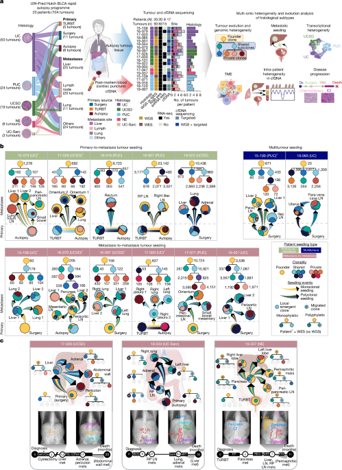
Specimens were obtained from 20 patients, including histopathologically normal tissue (n = 20, flash-frozen tissue), primary tumour samples (n = 24; 16 FFPE and 8 flash-frozen tissue) and 1–7 metastases per patient (n = 80, flash-frozen tissue). Details of tissue source, location, histology, among other information, for each sample are provided in Supplementary Table 1. Autopsy samples (n = 108), which included all normal, all metastatic and 8 primary tumour samples, were obtained within 11.5 h (median 3.7 h) of death as part of the rapid autopsy programme (Supplementary Table 1). For the logistical framework of the rapid autopsy programme, see Fig. 1a. A representative selection of the metastases observed at autopsy (excluding bone metastases) was chosen for sequencing, in addition to autopsy-derived primary tumour samples when available. Archival FFPE primary tumour samples (n = 16) included diagnostic (pre-treatment) TURBT (n = 5) and surgical specimens (n = 11) (Supplementary Table 1). All primary tumour and metastatic specimens selected for sequencing had more than 80% tumour cellularity based on genitourinary pathologist review (F.V.-L.). All normal tissues were confirmed to be normal by histology.

Study approval

All samples were obtained from patients with signed informed consent documents under the aegis of the Genitourinary Cancer Biorepository at the University of Washington (University of Washington IRB 2341). All 20 patients signed written informed consent for the rapid autopsy programme. Metastases and the primary tumour (if present) were identified and collected. In accordance with study protocols approved by the institutional review board, no metastatic biopsy samples collected from living patients were obtainable for use in this study.

Sectioning, H&E staining and pathologist assessment of tumour sections

All visceral metastases and matched primary tumour were embedded in Optimal Cutting Temperature compound (OCT; Tissue-Tek, Sakura Finetek) or FFPE. Haematoxylin and eosin (H&E) staining was completed as previously described^18,61. H&E-stained sections (5 µm) of the OCT-embedded and FFPE tissues were reviewed by an independent, dedicated genitourinary pathologist (F.V.-L.). The percentage of tumour, necrosis and histological subtypes were assessed and recorded for each section. Between one and ten sections per tumour or normal sample were assessed, depending on the size of the specimen available. The areas of >80% tumour were marked for macrodissection for DNA and RNA extraction purposes.

Histology was defined both at the patient level and the tumour (sample) level. All classifications were based on pathology assessment of FFPE H&E-stained specimens by pathologist (F.V.-L.) review based on the WHO classifications of ‘Urinary and Male Genital Tumours’ (5th edition)⁴. NE histology was further verified by synaptophysin positivity. PUC, UC-Sarc and UCSD tumours are UC with plasmacytoid, sarcomatoid or squamous differentiation, respectively. Patients and tumours were designated as non-UC if there was any evidence of variant histology. For patient-level histology, the histology was defined as a variant if there was evidence of subtype histology in any tumour in that patient (for example, if a patient had any tumour exhibiting any squamous differentiation, they were classified as UCSD). Patients 16-070, 17-030, 18-101 and 19-022 were designated UCSD because they had a mix of UC and UCSD tumours, whereas all tumours in patients 16-097 and 17-026 exhibited UCSD histology. Sample-level histology was defined for each tumour individually (for example, the primary tumour for patient 16-070 is UCSD, whereas their metastases are UC at the sample level). Further details on the percentage of histological subtypes in each tumour are given in Supplementary Table 1 (first sheet).

HER2 immunohistochemistry

FFPE sections (5 μm) were deparaffinized and rehydrated in sequential xylene and graded ethanol series¹⁷. HER2 protein expression was evaluated using a PATHWAY anti-HER2/neu (clone 4B5) kit on a Ventana BenchMark ULTRA platform (Ventana/Roche Tissue Diagnostics) following the manufacturer’s standardized protocols. Staining intensity (scored 0 to 3+) and the percentage of positive tumour cells were assessed by two pathologists (M.C.H. and E.S.).

Radiological assessment of CT scans

Clinical staging CT scans were requested for all 20 patients. A total of 59 scans (range 0–19 per patient) were available and acquired (Supplementary Table 2). These were scrubbed of all identifying metadata and the de-identified DICOM data were then uploaded to MIM (MIM Software, v.7.3.7, build O606-01). All CT scans were centrally reviewed by an independent radiologist as part of standard of care, and the de-identified radiology reports and scans were further evaluated by a radiation oncologist (O.Y.M.) to confirm the presence of the metastatic sites collected at autopsy. Primary and metastatic lesions corresponding to pathologically confirmed sites of disease at autopsy were circumscribed on all axial slices. Anterior–posterior plane projection digitally reconstructed radiographs were generated in MIM (Supplementary Fig. 2), with superimposed two-dimensional colour projections of all circumscribed radiographically identifiable malignant lesions (Fig. 1c and Extended Data Fig. 1e).

Corroboration of metastatic seeding

For each patient with metastasis-to-metastasis seeding (n = 9), the first available clinical staging CT scan after diagnosis was assessed for visible tumours to determine whether an initiating metastasis could be identified. For five patients in whom the early CT scan identified a first metastasis, subsequent CT scans were assessed to follow metastatic evolution. In patient 19-037, the sequenced peri-pancreatic LN corresponded to a portion of the RP LN visible in the CT scan. The remaining four patients were unable to be further assessed because of a lack of any staging CT scans (patient 15-108), all sequenced metastases were visible at the first CT scan (patients 16-097, 19-001) or there was a lack of clear correspondence between lesions visible on the first scan and metastatic sites collected at autopsy (patient 17-071) (Supplementary Fig. 2).

Determination of pre-ICI versus post-ICI metastasis

For each patient who underwent at least one full cycle of ICI treatment (n = 9; Supplementary Table 2), the CT scan that immediately preceded the start of ICI treatment was assessed for visible tumours. The time between the CT scan preceding ICI and the start of ICI was variable (median 16 days, range 2–260 days). For patient 19-022, the most recent CT scan available before ICI was 260 days before treatment, but clinical records confirmed that only the lung metastasis was observed before starting ICI treatment. The metastases already in place before ICI were designated as ‘pre-ICI metastases’, whereas metastases collected and sequenced at autopsy but not visible by CT before ICI were designated ‘post-ICI metastases’. Of the nine ICI-treated patients, there were three for whom all metastases were visible by CT before the start of ICI therapy. Six patients had both metastases visible pre-ICI and metastases that only appeared post-ICI. In total, 17 metastases were designated pre-ICI and 15 were post-ICI (Supplementary Table 3). Clonal composition (number and cellular prevalence of clones), metastatic seeding and metastatic site were compared between metastases seeded pre-ICI versus post-ICI.

We explored whether we could perform a similar retrospective seeding analysis for patients who received chemotherapy as we did for ICI treatment. Unfortunately, only three patients in our cohort (15-109, 17-020 and 17-026) received chemotherapy alone. Moreover, these three patients received chemotherapy early in the disease course; therefore, no metastases could be confirmed by CT scans before treatment.

Tumour volume calculations

Tumour volumes (in cubic centimetres) were calculated in MIM from patients’ last CT scan before death and exported in site-specific tabular format for subsequent correlative analyses.

Blood collection and fractionation from autopsy and healthy donors

Cardiac or venous blood collection was performed within 2.8–11.5 h of death, at the start of the rapid autopsy, using a 16–18 gauge needle and 20–50 cc syringes into Tiger Top (serum) or Purple Top (plasma) blood collection tubes and spun at 1,600g for 15 min. Supernatant plasma or serum were aliquoted using a Serum Bank pipette into 560–600 μl aliquots and stored at –80 °C until cfDNA extraction. Healthy donor plasma was purchased from Research Blood Components (no. 1-009, Fresh Plasma Single Donor 10 ml). Blood was collected in Cell-free DNA BCT Streck tubes and plasma was separated by centrifugation of whole blood at 1,600g for 10 min at room temperature. The upper plasma layer was removed, leaving the buffy coat undisturbed. Plasma was shipped on dry ice and stored at –80 °C until cfDNA extraction.

cfDNA extraction from plasma and serum

cfDNA was extracted using a QIAamp Circulating Nucleic Acid kit (Qiagen). After thawing 0.5–1.5 ml plasma or serum on ice, samples were spun at 15,000g for 10 min at room temperature. Supernatant was removed, avoiding disrupting any remaining pellet, and processed according to the manufacturer’s instructions, eluting cfDNA with 55 μl Buffer AVE. cfDNA concentration was quantified using a Qubit 1× dsDNA High Sensitivity Assay kit (Thermo Fisher Scientific, Q33230) on a Qubit 4 Fluorometer. cfDNA quality and fragment-size distribution were assessed from 3 μl (range 100–4,000 pg μl^–1) cfDNA run with an Agilent Cell-free DNA ScreenTape assay (Agilent Technologies) on an Agilent 4200 TapeStation system following the manufacturer’s instructions.

cfDNA sequencing

Seventeen patients had post-mortem cfDNA samples available from plasma (n = 7) or serum (n = 10), with high cfDNA yields (median 440 ng ml^–1) and detectable ctDNA of ≥3% TFx (median 5.9%). Ultralow-pass (ULP) WGS was performed for all samples. Deeper WGS and/or TP was subsequently performed on selected samples based on the estimated TFx.

ULP library preparation

ULP library preparation and sequencing were performed by Broad Clinical Labs for both plasma and serum samples. Initial cfDNA input was normalized to be within 25–52 ng in 50 μl TE buffer (10 mM Tris-HCl 12 mM EDTA, pH 8.0) according to PicoGreen quantification, with no shearing of cfDNA before library construction. Library preparation was performed using a commercially available kit (KAPA HyperPrep kit with Library Amplification product KK8504, KAPA Biosystems) and xGen UDI-UMI duplex adapters (Integrated DNA Technologies (IDT)). Unique 8-bp dual index sequences embedded in the p5 and p7 primers (IDT) were added during PCR. Enzymatic clean-up was performed using Beckman Coulter AMPure XP SPRI beads (Beckman Coulter, A63880), with elution volumes reduced to 30 μl to maximize library concentration. Library quantification was performed using an Invitrogen Quant-It broad range dsDNA quantification assay kit (Thermo Fisher Scientific, Q33130) with 1:200 PicoGreen dilution. Following quantification, each library was normalized to a concentration of 35 ng µl^–1 using Tris-HCl, 10 mM, pH 8.0.

ULP library pooling and sequencing

In preparation for ULP libraries, approximately 4 µl of the normalized library was transferred into a new receptacle and further normalized to a concentration of 2 ng µl^–1 using Tris-HCl, 10 mM, pH 8.0. Following normalization, up to 95 ULP WGS samples were pooled together using equivolume pooling. The pool was quantified by qPCR and normalized to the appropriate concentration to proceed to sequencing. Cluster amplification of library pools was performed according to the manufacturer’s protocol (Illumina) using Exclusion Amplification cluster chemistry and NovaSeq SP flow cells. Flow cells were sequenced on a NovaSeq 6000 Sequencer using the XP workflow and a v.1.5 300 cycle NovaSeq SP kit. Each pool of ULP whole-genome libraries was run on one lane using paired 151 bp runs.

TFx estimation using ichorCNA

ULP WGS data were analysed using ichorCNA⁶² (https://github.com/GavinHaLab/ichorCNA; commit ID: d31ed52) to estimate the TFx. Settings for hg38 build and 1 Mbp bin size were used. The final configuration file is available from GitHub (https://github.com/GavinHaLab/BLCA-subtype-evolution-paper). The TFx estimate was used to inform follow-on deeper WGS and TP sequencing.

Deep WGS from ULP libraries for high TFx ctDNA samples

Following initial ULP sequencing, selected ULP libraries with a TFx of ≥8% underwent further sequencing. Libraries were initially normalized to 2 ng µl^–1, pooled, then quantified by qPCR using a KAPA Biosystems kit that uses probes specific to the ends of the adapters. On the basis of the qPCR results, the libraries were adjusted to 2.2 nM before proceeding to the next sequencing stage using an automated Agilent Bravo liquid-handling platform. Pools were denatured with sodium hydroxide, diluted using an Illumina-provided pre-load buffer and transferred to a uniquely-barcoded 8-lane strip tube with a Hamilton Starlet liquid handler. Strip tubes were loaded into a 300 cycle NovaSeq X 25B kit and the run was initiated with a 151-bp end, dual-indexed read structure. On the basis of the pool size, the number of lanes was calculated to ensure samples reached the desired mean coverage.

PanCancer TP sequencing

After ULP library construction, in-solution hybridization and TP capture were performed using the relevant components of a XGen hybridization and wash kit (IDT) following the manufacturer’s suggested protocol, but with several exceptions. A set of 12-plex pre-hybridization pools were created. These pre-hybridization pools were created by equivolume pooling of the normalized libraries, human COT-1 and IDT XGen blocking oligonucleotides. The pre-hybridization pools underwent lyophilization using Biotage SPE-DRY. After lyophilization, custom PanCancer bait (Twist Biosciences) along with hybridization master mix were added to the lyophilized pool before resuspension. Samples were incubated overnight. Library normalization and hybridization setup were performed on a Hamilton Starlet liquid-handling platform, whereas target capture was performed on an Agilent Bravo automated platform. After capture, PCR was performed to amplify the capture material. After post-capture enrichment, library pools were quantified by qPCR (automated assay on the Agilent Bravo) using a kit purchased from KAPA Biosystems with probes specific to the ends of the adapters. On the basis of qPCR quantification, pools were normalized using a Hamilton Starlet to 2 nM and sequenced using Illumina sequencing technology.

TP cluster amplification and sequencing

Cluster amplification of library pools was performed according to the manufacturer’s protocol (Illumina) using Exclusion Amplification cluster chemistry and HiSeqX flow cells. Flow cells were sequenced on v.2 Sequencing-by-Synthesis chemistry for HiSeqX flow cells. The flow cells were then analysed using RTA (v.2.7.3 or later). Each pool of libraries was run on paired 151 bp runs, reading the dual-indexed sequences to identify molecular indices and sequenced across the number of lanes needed to meet coverage for all libraries in the pool.

Tissue WES and WGS

WES was performed as previously described¹⁶. WGS of flash-frozen normal control tissue (30× WGS) and FFPE or flash-frozen tumour samples (60× WGS) were performed by Broad Clinical Labs. gDNA derived from FFPE samples for a subset of primary tumours was sequenced using Human Whole Genome Sequencing PCR Plus (v.1.1–v.1.3), whereas a PCR-free method was used for gDNA from flash-frozen tissue. An aliquot of gDNA (100 ng in 50 µl for FFPE samples, 350 ng for flash-frozen samples) was used as input into DNA fragmentation by acoustic shearing using a Covaris focused-ultrasonicator, targeting 385 bp and 350 bp fragments, respectively. Following fragmentation, additional size selection was performed using SPRI cleanup. Library preparation was performed using a commercially available kit (KAPA Hyper Prep with Library Amplification Primer Mix, product KK8504, KAPA Biosystems) and with palindromic forked adapters using unique 8-bp index sequences embedded in the adapter (purchased from Roche). For FFPE samples, the libraries were then amplified using 10 cycles of PCR. Following sample preparation, libraries were quantified by qPCR (kit purchased from KAPA Biosystems) with probes specific to the ends of the adapters on an automated Bravo liquid-handling platform (Agilent). On the basis of qPCR quantification, libraries were normalized to 2.2 nM and pooled into 24-plexes. Sample pools were combined with NovaSeq Cluster Amp Reagents DPX1, DPX2 and DPX3 and loaded into single lanes of a NovaSeq 6000 S4 flow cell using a Hamilton Starlet liquid-handling system. Cluster amplification and sequencing were performed on NovaSeq 6000 instruments using sequencing-by-synthesis kits to produce 151 bp paired-end reads. Output from Illumina software was processed using the Picard data-processing pipeline to generate BAM files containing demultiplexed, aggregated aligned reads.

TURBT WGS library preparation and sequencing

Sample processing for FFPE TURBT specimens was performed in similar manner to the FFPE primary samples. Tumour regions were macrodissected to achieve >80% tumour content, and dual DNA and RNA extraction was carried out at the Fred Hutchinson Cancer Center core facility. For two patients (17-020 and 17-026), normal tissues that were originally sequenced by WES were re-processed for WGS to serve as controls for the WGS TURBT samples, following the same protocol. FFPE tumour DNA and flash-frozen normal DNA were quantified using an Invitrogen Qubit 2.0 Fluorometer (Thermo Fisher Scientific). For library preparation, 100 ng DNA per sample was fragmented to a target size of 400 bp using a Covaris LE220-plus focused ultrasonicator. Sequencing libraries were then prepared from the fragmented DNA using a xGen cfDNA & FFPE DNA Library Prep v2 MC kit (IDT) in combination with xGen UDI indexing primers (IDT). Library quantification was performed using an Invitrogen Qubit 2.0 Fluorometer, and fragment size distribution was assessed using an Agilent 4200 TapeStation (Agilent Technologies). Individual libraries were pooled in 8-plex at weighted molar concentrations based on DNA type. Sequencing was conducted on an Illumina NovaSeq X Plus system (Illumina) across two lanes of a 25B-300 flow cell using a paired-end 150 bp read configuration, with an average sequencing output per library of 837 million read pairs (range 711–1,107 million).

Bulk tumour RNA-seq

For flash-frozen autopsy samples (n = 74), RNA was isolated from OCT-embedded specimens using a combination of RNA STAT-60 reagent (Tel-Test) and a RNeasy Mini kit (Qiagen), with an in-solution DNase treatment step included before purification. For FFPE surgical samples (n = 8), RNA was isolated using an AllPrep DNA/RNA FFPE kit (Qiagen). RNA quality was assessed by measuring the RNA integrity number using an Agilent Bioanalyzer (Agilent Technologies). Sample 18-016_G2 was excluded from bulk RNA-seq analysis owing to a low RNA integrity number score of extracted RNA. For RNA-seq, libraries were generated from 300 ng total RNA using an Illumina TruSeq RNA Exome Sample Prep kit, following the standard protocol (Illumina). The resulting barcoded libraries were pooled and sequenced on an Illumina HiSeq 2500 platform to produce 50-bp paired-end reads.

snRNA-seq

snRNA-seq was performed by Singulomics as follows. Nuclei were isolated from OCT-embedded frozen human BLCA tissue samples, and 3′ single-cell gene expression libraries (Next GEM v.3.1) were constructed using the 10x Genomics Chromium system. Libraries were sequenced with around 200 million 150-bp paired-end reads per sample on an Illumina NovaSeq X Plus. The sequencing reads were analysed using human reference genome GRCh38 with Cell Ranger (v.7.1.0). Introns were included in the analyses.

Cell culture experiments

Cell lines used in this study were SW780, HT1376, BFTC905 and UBLC1 BLCA cells. All cell lines were sourced from the American Type Culture Collection, authenticated using STR profiling and tested mycoplasma negative. Each cell line was cultured in DMEM high-glucose and l-glutamine medium (Gibco 11965-092) supplemented with 10% FBS, 1% penicillin–streptomycin, 1% l-glutamine and 1% MEM non-essential amino acids. Cell lines were cultured in an incubator at 37 °C with 5% CO₂.

Western blotting

Cells were treated in 10 cm dishes with 5 µM cisplatin or 1 µM MMC (Sigma, M5353) for 24 h before collection for western blotting. Cell pellets were lysed using RIPA buffer (Fisher Scientific) supplemented with protease and phosphatase inhibitors (Sigma). Equivalent amounts of protein per sample (5–40 μg depending on the target) were run on a polyacrylamide gel and transferred to a PVDF membrane. Proteins were detected using respective primary and HRP-conjugated secondary antibodies, including rabbit anti-FANCD2 (Abcam 108928 1:1,000), mouse anti-FANCF (Santa Cruz sc-271952 1:500), mouse anti-tubulin (Sigma-Aldrich T8203 1:1,000), rabbit anti-vinculin (Cell Signaling Technology 13901S 1:1,000), goat anti-rabbit (Invitrogen 31460 1:5,000) and goat anti-mouse (Invitrogen 31430 1:5,000). Quantification of images was performed in ImageJ.

siRNA-mediated FANCF knockdown

FANCF knockdown was performed using siRNA transfection in the FANC-high BLCA cell line SW780. Cells were seeded in parallel in 96-well plates (3,000 cells per well) for live-cell imaging assays and in 6-well plates (2.5 × 10⁵ cells per well) for RNA and protein analyses. Cells were transfected the following day using Lipofectamine RNAiMAX (Thermo Fisher Scientific) according to the manufacturer’s instructions (forward transfection), with either non-targeting control (Dharmacon D-001810-10-05) or FANCF-targeting (Dharmacon L-014206-00-0005) siRNA SMARTpools. At 24 h after transfection, cells plated in 6-well plates were collected for RNA extraction to assess knockdown efficiency by qPCR. Protein lysates were collected at 48 h after transfection for immunoblot validation.

Lentiviral overexpression of FANCF

FANCF overexpression was achieved by lentiviral transduction in the FANC-low BLCA cell line UBLC1. Plasmids encoding empty vector control (pCR1265) or FANCF (pCR1446) were obtained from Addgene⁶³. Lentivirus was produced in HEK293T cells via calcium phosphate (CaCl₂–HBSS) transfection using third-generation packaging plasmids. Viral supernatant was collected 72 h after transfection, filtered through a 0.45 μm membrane, aliquoted and stored at −80 °C before use. UBLC1 cells were transduced with lentiviral supernatant overnight without transduction enhancers. Following transduction, cells were selected with geneticin (G418; 1 mg ml^–1) for 7 days to establish stable expression. Stable expression of FANCF was confirmed by both qPCR and immunoblotting.

qPCR

Total RNA was extracted from cell pellets using a RNeasy Plus Mini kit (Qiagen). iScript Reverse Transcription Supermix (Bio-Rad) was used to reverse-transcribe cDNA from equal volumes of RNA across samples. qPCR was performed using SsoAdvanced Universal SYBR Green Supermix (Bio-Rad) for FANCF (5′-GGTGGCGGCTAGTCACTAAA-3′, 5′-GCTAGTCCACTGGCTTCTGG-3′) and GAPDH (5′-ACCCACTCCACCTTTGAC-3′, 5′-ATGAGGTCCACCACCCTGTTG-3′).

Immunofluorescence staining for γH2AX

Cells (5 × 10⁴) were seeded onto poly-l-lysine-coated glass coverslips in 24-well plates and allowed to adhere overnight. The following day, cells were treated with cisplatin at doses approximating the IC₅₀ for each cell line. FANC-high cells (SW780) were treated with 10 μM cisplatin, whereas FANC-low cells (UBLC1) were treated with 5 μM cisplatin. Cells were exposed to cisplatin for 3 h, after which the drug-containing medium was removed and replaced with fresh medium. Cells were fixed at 0, 4, 24 and 48 h following drug removal. For immunofluorescence staining, cells were rinsed briefly with PBS and fixed with 4% paraformaldehyde in PBS for 10 min at room temperature. Fixation was quenched using 500 mM Tris and 125 mM glycine for 5 min, followed by washing with PBS. Cells were permeabilized with 0.5% Triton X-100 in TBS for 5 min and washed once with PBS. Samples were blocked using MaxBLOCK (Active Motif) for 1 h at 37 °C, followed by 2 washes with TBS containing 0.1% Tween-20 (TBST). Cells were incubated with a primary antibody against γH2AX (mouse; Sigma, 05-636; 1:4,000) diluted in 1% BSA in TBST for 1 h at room temperature. Coverslips were washed twice with TBST and incubated with Alexa Fluor 633 goat anti-mouse secondary antibody (ThermoFisher, A-21052; 1:1,000) for 1 h at room temperature in the dark. Following secondary incubation, cells were stained with DAPI (2 μg ml^–1 in TBST) for 10 min, washed twice with TBST and rinsed once with water to remove residual salts. Coverslips were mounted onto glass slides using ProLong Diamond Antifade mountant (Thermo Fisher Scientific) and allowed to cure at room temperature before imaging. Slides were stored at 4 °C. Images were acquired with a Leica Stellaris 8 scanning confocal microscope equipped with a 40×/1.3 NA oil HC PL APO CS2 objective. A total of 100 z stacks were acquired for each slide. DAPI and Alexa Fluor 594 were imaged using 420–504 nm and 600–750 nm detection windows, respectively.

Images were analysed using Imaris (v.11) by first segmenting nuclei based on DAPI staining using the machine-learning surface tool with an estimated diameter of 8 μm in UBLC1 cells and 7 μm in SW780 cells. Nuclei with a median γH2AX intensity of more than 15 were excluded from further analyses, as these were probably dying cells. The median number of nuclei per image after filtering was 1,130 (minimum = 537, maximum = 1,395). γH2AX foci were identified in nuclei using the spots tool with an estimated diameter of 0.4 μm, minimum mean intensity of 15 and minimum quality of 3.5. The number of foci per nucleus was calculated using the Imaris cells tool.

Cell growth and death assays

Cell lines were plated at between 5,000 and 15,000 cells per well in 96-well plates to achieve starting densities of approximately 30%. The next day, the cell medium was changed to include 0–20 µM cisplatin (0, 1, 2.5, 5, 10 and 20 µM doses) or 0–10 µM MMC (0, 0.05, 0.10, 0.5, 1, 2.5, 5 and 10 µM doses) and, for cell death experiments, 250 nM of IncuCyte Cytotox dye (Sartorius). Each cell line was plated in four or five technical replicate wells per condition. Cells were moved immediately after treatment to an IncuCyte S3 or IncuCyte SX5 platform for continuous imaging and confluence analyses. Cells were imaged over the course of 72 h, and IncuCyte software (v.2023A Rev1, Sartorius) was used to measure changes in confluence and to count dead and dying cells (fluorescent puncti from Cytotox dye) in each well at each time point.

For cell growth analyses, the cell confluence was normalized to the starting confluence for each well. To calculate IC₅₀ values, dose–response curves were fit using a four-parameter log-logistic (LL.4) function and applied to these normalized growth values as a function of cisplatin dose. Curve fitting was performed using the drm function of the R package drc (v.3.0-1). The auc function from the R package MESS (v.0.6.0) was used to calculate AUC values from the normalized confluence values.

For cell death analyses, the count of dead and dying cells (Cytotox fluorescent puncti) in each well was normalized to the cell confluence of that well to obtain a representation of the proportion of dying cells. The auc function of the R package MESS (v.0.6.0) was used to calculate AUC values from the normalized dead cell values.

Sequence alignment

DNA sequencing reads were aligned to the GRCh38 human genome using BWA-MEM (v.0.7.17). Alignments were then sorted and indexed using samtools (v.1.10), and duplicates were marked using picardtools MarkDuplicates (v.2.18.29). Finally, alignments were subjected to base quality score recalibration using BaseRecalibrator and ApplyBQSR from GATK (v.4.1.8.1). Read counts and the per cent of properly mapped reads were collected using CollectAlignmentSummaryMetrics, and CollectWgsMetrics was used to gather the mean coverage (GATK v.4.1.8.1). These steps generated recalibrated BAM files that were used for further analyses. For the WES samples, metrics were collected using the tool HsMetrics and an exome capture bedfile. The healthy donor plasma samples were processed using the same approach as described above to generate the final BAM files for analyses. The sequencing metrics were computed using CollectWgsMetrics.

BLCA-driver gene list creation

We compiled a total of 128 known potential metastatic BLCA-driver genes. First, we used the IntOGen database⁶⁴ to identify a list of 95 genes from 8 cohorts comprising 867 samples. Next, to enhance this list, we manually incorporated 24 additional genes identified by the Hartwig Medical Foundation. Finally, we included nine genes reported in BLCA literature as commonly affected in metastatic BLCA^{6,65,66,67,68}. This curated list of 128 driver genes was used for all downstream analyses.

Next, we annotated the functional roles of these 128 genes in BLCA by using the Cancer Gene Census⁶⁹ and OncoKB⁷⁰ databases. For each gene, if both databases listed the gene as a tumour suppressor or as an oncogene, then this annotation was used. If the databases differed with each other, did not list an annotation or listed multiple conflicting annotations, then the gene was designated ‘Other’. The driver genes and annotations that were used for all analyses are provided in Supplementary Table 4.

Somatic mutation consensus calling

To identify high-confidence somatic mutations from tumours, we implemented a consensus-based variant calling strategy using four somatic callers: Mutect2 (ref. ⁷¹), Strelka2 (ref. ⁷²), VarScan2 (ref. ⁷³) and MuSE⁷⁴. All tools were run in paired tumour–normal mode, leveraging matched normal samples to exclude germline variants. For Mutect2, we also constructed a panel of normals to remove recurrent technical artefacts. Different panels of normals were generated for WES (n = 7) and WGS (n = 13) cohorts using the ‘Create a Panel of Normals’ workflow in GATK⁷⁵.

Genomic variant annotation was conducted using ANNOVAR (v.2020-06-07)⁷⁶ with the table_annovar.pl script to functionally interpret variants identified in the study. The analysis was performed using the human genome build GRCh38 (Broad version). The input VCF file was annotated against a comprehensive set of databases, including RefSeq genes (refGene) for gene-based annotation and cytogenetic band information (cytoBand) for region-based annotation. The variant frequency in the population and functional scores were annotated using clinical databases, including the NHLBI-ESP 6500 dataset (esp6500siv2_all), dbSNP (v.144 and v.150; avsnp144 and avsnp150), the 1000 Genomes Project (ALL.sites.2015_08), gnomAD genome and exome datasets (gnomad_genome and gnomad_exome), ExAC (v.0.3; exac03), ClinVar (release 20190305), InterVar (release 20180118) and dbNSFP (v.3.3a) for functional prediction scores, and gnomAD (v.3.1.2) genome data (gnomad312_genome) and COSMIC (v.70) for somatic mutation data. The annotation process used the –vcfinput flag to accept VCF format input and the -polish option to refine annotations. Variants with missing annotations were marked with a dot using the -nastring option, and intermediate files were removed after processing using the -remove flag.

Criteria for high-confidence consensus mutation filtering

A SNV was considered high-confidence if it was identified by at least two out of the four callers and met the following somatic call filtering criteria: (1) the matched normal sample contained ≥8 reference reads; (2) the tumour sample had ≥14 total reads and ≥5 mutant reads; (3) the tumour variant allele frequency (VAF) was ≥1%; and (4) the normal VAF was ≤5%. The frequency of SNVs greater than 10% in gnomAD or ExAC databases were filtered out to generate the final high-confidence somatic SNV set for downstream analyses.

For calling indels, we used, Mutect2, Strelka2 and SvABA⁷⁷, also in paired mode with the corresponding matched normal. Indels were retained only if they were detected by all three callers and the Mutect2 tumour VAF was >1%. Mutations with a frequency greater than 10% in gnomAD or ExAC databases (to exclude common population variants) were filtered out to generate the final consensus indel call set for downstream analyses. Last, for all analyses involving somatic mutations, four primary tumour samples, 17-047pD10, 18-101M3, 18-120pA14 and 19-044pB11, were excluded because they had a tumour purity of <20% or had poor-quality FFPE DNA sequencing data.

Analysis of positive and negative selection

We used the dNdScv R package (v.0.010, https://github.com/im3sanger/dndscv) to estimate dN/dS ratios across the cohort, which enabled detection of positive or negative selection in a set of mutations⁷⁸. This method applies maximum-likelihood modelling of synonymous and non-synonymous mutations, accounting for gene-specific background mutation rates, sequence context and trinucleotide mutational signatures. All somatic mutations were included, stratified by founder, shared and private status. Analyses were performed separately for BLCA-driver genes and all other genes (‘All genes’) and only the global dN/dS estimates are reported (Supplementary Fig. 3).

CNA analysis

Copy number calls

To identify CNAs, we used the TITAN⁷⁹ (v1.15.0) pipeline (https://github.com/GavinHaLab/TitanCNA_SV_WGS; commitID: bedbd76). TITAN-derived results were manually curated to confirm the optimal solution for each sample and are shown in Supplementary Table 1. The ploidy and purity of each tumour were derived from these TITAN optimal solutions. Default settings were used, except the bin size for WES data, which was set to 50 kb windows, whereas for WGS data, 10 kb windows were used.

Gene overlap of tumour CNAs

To construct a gene-level CNA matrix, a copy number status was assigned to each gene on the basis of its overlap with TITAN-derived copy number segments and gene coordinates from Ensembl BioMart (GRCh38.p12). To enable consistent comparisons across tumour samples, gene-level copy numbers were further normalized to account for sample-specific ploidy. First, the approximate ploidy was computed as the median copy number across all genes in the sample. Then, for each gene, its copy number was divided by this approximate ploidy to produce a normalized copy ratio (c_gene). CNAs were classified as gains if c_gene > 1.3, losses if c_gene < 0.66 and neutral if 0.66 ≤ c_gene ≤ 1.33. The resulting gene-level, ploidy-adjusted copy number matrix was used for downstream analyses. The same ploidy-based normalization and classification approach was applied to the validation cohorts (Hartwig Medical Foundation and The Cancer Genome Atlas (TCGA)) for copy number comparisons.

Founder, shared and private copy number clonality status

To classify the clonality of CNAs as being in founder, shared or private clones, we analysed gene-level CNAs across multiple tumours in each patient. Each gene was assigned either loss, neutral or gain status (as described above), and a founder, shared or private status based on whether the event was present with the same alteration status in all samples of the patient (founder), in multiple but not all samples (shared) or unique to a single sample (private).

Patient-level copy-number status and fraction of genome altered estimation

For each tumour, we divided the genome into 1 Mb bins and, for each bin, calculated the median copy number across all overlapping CNA calls. This size of binning enabled joint analyses of CNA results for WGS and WES, which were originally analysed using different bin sizes. Next, the copy number for each bin was divided by the median corrected copy number from TITAN across all 1 Mb bins in the sample, which produced a normalized copy ratio (c_bin). CNAs were classified as gains if c_bin > 1.3, losses if c_bin < 0.66 and neutral if 0.66 ≤ c_gene ≤ 1.33. The fraction of genome altered was calculated for each patient by counting the number of 1 Mb bins showing a copy number gain or loss and dividing the total number of all bins in that patient.

For all CNA-based analyses, six samples were excluded, including 17-030pM9 and 19-022pJ13-B, as well as the four samples already excluded for the mutation analyses, owing to high variability in copy number profiles.

Mutation clonality analysis

To assess cellular prevalence, defined as the proportion of tumour cells with a given somatic mutation, we used PyClone-VI⁸⁰ (v.0.1.1; https://github.com/Roth-Lab/pyclone-vi;commit ID: 6607ea1), a Bayesian clustering framework used to infer clonal population structure by grouping mutations with similar cellular prevalence. This analysis incorporated consensus SNV, indels, CNAs and matched tumour purity and ploidy estimates from TITAN. For each patient, we began by merging SNVs and indels from all available tumour samples in a patient into a unified mutation list. In cases when the primary tumour samples were FFPE, we applied an additional filtering step whereby we retained only the mutations that were also present in at least one metastatic tumour from the same patient. This step was done to mitigate the impact of sequencing artefacts and false positives in FFPE-derived data. As a result, mutations found exclusively in FFPE primary tumours were not considered in the mutation clonality analyses.

Following the generation of the unified mutation list, we extracted allelic read counts for each SNV using the following prioritization: (1) if an SNV was present in the tumour sample of the consensus somatic SNV set, then read counts were obtained from the corresponding variant caller in the following order of priority: Mutect2, Strelka2, MuSE and VarScan; or (2) if a SNV was not present in the tumour sample of the consensus set, allelic read counts were obtained using CollectAllelicCounts from GATK. For indels, read counts were extracted using bam-readcount (https://github.com/genome/bam-readcount, commit ID: c7c76e6). A final file was created to contain read counts for both SNVs and indels, as well as major and minor allele copy numbers across all tumours for a patient.

This final file was used as input for the fit function in PyClone-VI. The beta-binomial model was used with default parameters, except we specified a maximum of 7 clusters, 10,000 iterations and a burn-in of 1,000.

Phylogenetic tree reconstruction using LICHeE

Phylogenetic reconstruction was performed using LICHeE⁸¹ (v.1.0) (https://github.com/viq854/lichee; commitID:26c2a70) with the mutation clusters derived directly from PyClone-VI. For each patient, we generated two input files: a mutation file with SNV and indel presence or absent, and a cluster file with the cellular prevalence (C.P. from PyClone-VI) profiles across tumour samples. We ran LICHeE in cellular prevalence mode (-cp) with an error margin of 0.4 to retain all clusters. We specified the following parameters: -maxVAFAbsent 0.0, -minVAFPresent 0.5, -maxClusterDist 0.2, -minRobustNodeSupport 2, -minClusterSize 20, -minPrivateClusterSize 1 and -e 0.4. Before tree construction, we excluded clusters containing fewer than 20 mutations or with a cellular prevalence below 0.03 to omit small clonal clusters with less mutation support. For each patient, we selected the top-scoring phylogenetic tree based on the tree with the minimum sum of squared deviations.

Founder, shared and private clonal cluster definitions

The resulting trees represented subclonal evolutionary relationships^82,83. Clusters were classified on the basis of their average cellular prevalence and distribution across samples (Supplementary Table 3). A cluster was designated as founder if it had the highest average cellular prevalence (median = 0.99) in the patient and was consistently detected across all samples (minimum average cellular prevalence = 0.61). Shared clusters were present in more than one sample but had a lower average cellular prevalence than the founder cluster in that patient. Private clusters were restricted to a single sample and exhibited a non-zero cellular prevalence in that sample.

Visualization of clones

We visualized the trees using the LICHeE Java viewer and exported them as annotated DOT images and pdfs for downstream analyses. To visualize subclonal architecture in the context of phylogenetic structure and cellular prevalence, we used the R package cloneMap⁸⁴ to make octagon-shaped visualizations of each tumour (https://github.com/amf71/cloneMap; commitID: 7628d70). Input data included mutation clusters and lineage relationships inferred by LICHeE, along with cellular prevalence estimates from PyClone-VI. These were formatted according to cloneMap specifications, and the tool was executed using default parameters. Clone sizes were scaled according to sample-specific cellular prevalence values, whereas spatial positioning of clones reflected their inferred phylogenetic relationships. Final clone maps were exported as high-resolution vector graphics for integration into downstream figure panels, including those illustrating metastatic seeding patterns.

Metastatic seeding analysis using MACHINA

To infer metastatic seeding patterns and clonal migration histories, we applied MACHINA⁸⁵ (https://github.com/raphael-group/machina; commit ID: ac71282; v.1.2), a computational tool designed to reconstruct tumour seeding across primary and metastatic sites. MACHINA metastatic seeding analysis was performed on 16 out of of the 20 patients; 4 patients (17-047, 18-101, 18-120 and 19-044) were excluded from this analysis as their primary tumours either had estimated tumour purity <20% or poor-quality FFPE DNA sequencing data. The input data included mutation clusters and clonal assignments derived from LICHeE-generated trees, formatted according to the input requirements of MACHINA.

MACHINA was run using both the parsimonious migration history (pmh) and pmh with tumour reseeding (pmh_tr) models to account for single and multiple seeding events between tumour sites. Migration inference was performed under an unrestricted migration model that allowed the following seeding types: primary seeding (seeding from the primary tumour); metastatic seeding (seeding to other sites); metastasis-to-metastasis seeding; and reseeding.

For trees that included polytomies (that is, LICHeE clusters with three or more descendant clones), we favoured solutions from the pmh_tr model. To select the most parsimonious solution, we first identified those with the lowest total number of migration and comigration events. If multiple solutions had the same total, we prioritized the one with fewer migration events, assuming that migration is less frequent. If a tie remained, we selected the solution in which the most recent common ancestral node (in the LICHeE tree) had the highest cellular prevalence, thereby reflecting a more dominant seeding clone. Candidate clone trees were evaluated for each patient and, when available, CT scans were used to help confirm the selected solutions.

Migration trees and clonal relationships were visualized using Graphviz. MACHINA was run on a high-performance computing cluster using Gurobi (v.11.0) with a WLS licence.

Multivariate Cox regression models that included known prognostic factors of age, sex and histology were used to assess the relationship between polyclonality of seeding (the mean number of migrating clones across all metastatic seeding events in each patient) and patient survival from first metastasis to death. The time that the patient’s first metastasis was observed by CT scan was set to t₀ to reduce confounding from the variable interval of disease-free survival from diagnosis to first metastasis. For one patient who presented with metastases at diagnosis, we use diagnosis as the time of first metastasis, although there is uncertainty as to when these tumours may have first arisen in the patient. To compute the mean seeding polyclonality metric, we used the following equation. Let c_m,p be the number of clones required to seed metastasis m in patient p. Then, the mean number of clones per seeding event across M total metastases in the patient p was defined as \(\overline{{C}_{p}}=\left({\sum }_{m}^{M}{c}_{m,p}\right)/M\). Patient 16-070 was excluded from this analysis owing to being a statistical outlier in survival from first metastasis to death (z score = 3.5).

SV analysis

SV consensus calling

To establish a set of high-confidence consensus SVs, we used three tools, SvABA⁷⁷, Manta⁸⁶ and GRIDSS⁸⁷, to generate a consensus list. A SV event was retained for downstream analyses only if it was detected by at least two out of the three tools. A SV event identified by different callers were considered the same event if each of their two breakpoints overlapped in a 1 kbp window. This created a set of consensus SVs that were merged across callsets made by each tool. Next, SVs were classified as insertions, deletions, duplications, translocations or inversions on the basis of their breakpoint orientations. We further refined this list by retaining only SVs greater than 1 kbp in length, thereby focusing on larger, potentially more impactful genomic alterations and not accounting for small deletions.

SVs with breakpoints located in the ENCODE⁸⁸ blacklist (https://github.com/Boyle-Lab/Blacklist) were excluded. A gene was considered transected (broken) by an SV if at least one of its breakpoints overlapped the gene based on the coordinates from GENCODE release 44 (GRCh38.p14; basic gene annotation, CHR regions).

For all SV-based analyses, six samples were excluded, including 17-030pM9 and 19-022pJ13-B, as well as the four samples already excluded for the mutation analysis, owing to high variability in copy number profiles.

Complex SV analysis

Complex SVs were detected using two tools: Junction Balance Analysis (JaBbA)²² and Amplicon Architect (AA)⁸⁹. For JaBbA, the tool was installed from GitHub (v.1.1, https://github.com/mskilab-org/JaBbA; commitID: e3dc184). JaBbA was run on a high-performance computing cluster using a Gurobi WLS licence and Gurobi (v.11.0). The consensus SV data in BEDPE format were used as junction inputs. For genome-wide coverage input, we used the tumour-to-normal coverage ratio generated by ichorCNA as part of the TITAN pipeline (bin size of 10 kbp) and used the default algorithm CBS for tumour–normal copy number segmentation input. The purity and ploidy estimates were provided from TITAN-curated solutions (Supplementary Table 1). All other parameters were kept at their default settings.

Complex SVs such as breakage–fusion–bridge cycles, double minutes, rigma, pyrgo and templated insertion chains were called on junction-balanced genome graphs and rds files from JaBbA using the companion package gGnome (v.0.1, https://github.com/mskilab-org/gGnome; commitID: ee19bea). Any simple SVs such as inversions, translocations and duplications detected from JaBbA were not used for analyses. gGnome was used to visualize certain complex SV events and to save the rds files generated by JaBbA as.txt files for further downstream analyses. We further manually curated the presence of these events by looking into the chromosome-level plots (Fig. 2i and Supplementary Fig. 4) and confirmed the presence or absence of complex SVs.

AA was run using the end-to-end wrapper AmpliconSuite-pipeline (v.1.2.2, https://github.com/AmpliconSuite/AmpliconSuite-pipeline; commitID: 7ae7f32), which enabled the detection and classification of focal copy number amplifications such as ecDNA and breakage–fusion–bridge events from WGS data. All relevant libraries and repositories for the GRCh38 reference genome were used.

AA identified focal amplifications by first defining seed intervals as genomic regions larger than 50 kb with a copy number greater than 4.5 and using a downsampling factor of 20. For FFPE samples, a downsampling factor of 1 was used to mitigate FFPE-associated sequencing artefacts. The resulting breakpoint graph was decomposed into simple and complex cycles to detect potential circular DNA structures, including ecDNA. We classified tumours by the presence or absence of ecDNA or breakage–fusion–bridge or complex SVs. Any linear amplifications (chromosomal) detected were not considered for analyses. If both chromosomal and ecDNA were present, patients were included in the ecDNA group.

Annotation and merging JaBbA and AA results

SV footprints identified by JaBbA and amplicons detected by AA were merged and unique events were retained. Merging was performed on the basis of a reciprocal overlap criterion: SVs were considered concordant if they shared at least 75% overlap in breakpoint coordinates or if the overlapping region encompassed at least 50% of the genes reported by either tool. To consolidate SVs across multiple tumour samples from the same patient, we applied the same merging criteria—75% breakpoint overlap or 50% gene overlap—thereby generating patient-level SV event counts. Each SV event was annotated for overlap with known BLCA driver genes: an event was classified as a driver complex SV if any breakpoint intersected a driver gene.

SV clonality analysis

Clonality of simple SVs such as insertions, deletions, duplications, inversions and translocations was assessed using SVclone⁹⁰ (v.1.1.3, https://github.com/mcmero/SVclone; commit ID: 93dafb2), a tool designed to estimate the cancer cell fraction (CCF) of somatic SVs from WGS data. The pipeline was run using default parameters unless otherwise specified in a single sample mode. Input data included high-confidence consensus somatic SV calls in VCF format and matched tumour–normal BAM files.

SVclone first annotates and filters SVs, then calculates VAFs by counting supporting and non-supporting reads at each breakpoint. These counts were adjusted for copy number and tumour purity (from TITAN) to estimate the CCF of each SV. SVs were then clustered on the basis of their CCFs to infer subclonal architecture.

Only SVs passing all quality filters and with sufficient read support (a minimum of 1 split and 1 discordant read) were included in downstream SV clonality analyses. Clusters with CCFs > 0.90 were considered clonal, whereas those with lower CCFs were classified as subclonal. To further obtain a SV CCF status per patient (SVclone is for single sample runs) we used our custom script, which merges the different SVs in tumours of a patient to obtain a final list of SVs with CCF for each patient. For each patient, we merged overlapping SV calls across that patient’s tumour samples using a 500 bp window in BEDPE format to produce a unified per-patient SV list. Each SV was then classified as founder if it was clonal and detected in every tumour, shared if it occurred in two or more but not all tumours, or private if it was unique to a single tumour.

Visualization of somatic alterations (comut)

Somatic alterations for curated BLCA-driver genes were visualized using the Python package comut⁹¹ (v.0.0.3, https://github.com/vanallenlab/comut, commitID: 0ee1408). Mutations were shown on the basis of founder, shared or private clonal status. For each SNV and indel, mutations that did not qualify as being present were defined as one of the following: (1) below threshold (when a mutation is clustered by Pyclone-VI as being in a shared or founder cluster present in the tumour, but the sample itself does not have sufficient evidence for the mutation (it was filtered out based on the criteria listed in criteria for high-confidence consensus mutation filtering)); (2) no mutation (for any sample in a patient for whom the mutation was not found in the consensus SNV call set, despite having a read depth providing sufficient statistical power (≥80%)); or (3) no power (the depth at the mutation site did not provide sufficient power). The power was estimated for SNVs based on a previously used approach¹⁶ that incorporates the total read depth at each SNV locus, tumour purity and ploidy. SNVs with a power estimate below 80% were considered to have insufficient power.

Classifying BLCA pathogenic alterations

To determine whether a mutation is pathogenic, we used a consensus-based approach that incorporated multiple predictive algorithms. Specifically, if any 3 or more of the following 11 predictors classify a mutation as deleterious, it was labelled as pathogenic: SIFT, PolyPhen-2 HDIV, PolyPhen-2 HVAR, MutationTaster, MutationAssessor, FATHMM, PROVEAN, MetaLR, M-CAP, ClinVar and FATHMM-MKL. In addition to these computational predictions, we also considered other forms of supporting evidence: the mutation is listed in the COSMIC (v.70) database and occurs in one of the128 BLCA driver genes; it is a splicing mutation affecting BLCA-driver gene; or it is a frameshift indel in a BLCA-driver gene.

This approach improved the identification of potentially pathogenic mutations by combining multiple lines of evidence, including predictive algorithms and biological context. CNAs were considered pathogenic only if the event was a gain in an oncogene or a loss in a tumour suppressor from the list of BLCA-driver genes. Any CNA in a BLCA gene that could not be classified as clearly oncogene or tumour suppressor was not considered as pathogenic. We classified any SV intersecting a BLCA-driver gene as pathogenic, even if only a single breakpoint fell in the driver gene. For analyses of clinical associations between pathogenic alterations and survival (time from diagnosis to death or metastasis), patient 17-047 was excluded as an outlier owing to markedly longer survival from diagnosis to death (9.5 years, z score = 2.8). Patient 19-004 was also excluded from these analyses as the sole case with a UC-Sarc histological subtype.

Mutational signature analysis of patient phylogenetic trees

Phylogenetic trees were constructed for each patient using LICHeE (v.1.0, see above). SNVs assigned to each node in the resulting phylogeny were then analysed using SigProfiler suite of tools to estimate the SBS mutational signature composition of each cluster or clone in the tree.

Mutational signature analysis was performed using SigProfilerAssignment⁹² (v.0.1.1, https://github.com/AlexandrovLab/SigProfilerAssignment; commit ID: 327fb93) SigProfilerAssignment was run on individual mutation clusters (clones) identified by PyClone-VI, which resulted in a distinct set of SBS signatures for each clone in a patient.

To achieve this, SNVs from each cluster were formatted into VCF files using a five-column format: chromosome, genomic coordinate, sample ID, reference allele and alternative allele. All sample VCFs were then processed collectively using SigProfilerAssignment⁹² (v.1.1.23) to extract mutational signatures and to generate a matrix of mutation counts across the 96 SBS patterns. Signature extraction was conducted across all samples and matched to known COSMIC (v.3.2) SBS reference signatures. A final signature refitting step was performed using a curated subset of COSMIC SBS signatures. Non-relevant chemotherapy-associated signatures (for example, SBS11 (temozolomide), SBS86 (unknown chemotherapy), SBS87 (thiopurine chemotherapy) and SBS42 (haloalkane exposure)) and UV-related signatures (SBS7a–d and SBS38) were excluded, which resulted in a set of 51 COSMIC (v.3.2) SBS signatures. One of the seven patients who did not receive platinum-based chemotherapy displayed a minor proportion of platinum-associated signatures (SBS31 + SBS35), which is probably an artefact owing to the low mutation count in this mutation cluster. Therefore, for these seven patients, SBS31 and SBS35 were also excluded, and refitting was performed separately to avoid such artefacts, which generated a final set of 49 signatures used for downstream analyses in this group (Supplementary Table 5).

Mutation signatures were grouped into aetiologies for analyses as follows: APOBEC (SBS2 + SBS13); Clock-like (SBS1 + SBS5); platinum chemotherapy (SBS31 + SBS35); and DNA repair deficiencies (SBS3, SBS6, SBS14, SBS15, SBS20, SBS21, SBS26, SBS30, SBS36 and SBS44).

Bulk tumour RNA-seq analysis

Raw sequencing reads were assessed for quality using FastQC (v.0.12.1). Using STAR2 (v.2.7.3a), RNA-seq reads were aligned to the UCSC hg38 genome assembly and quantified for gene-level expression using HTSeq (v.0.11.1) against the gencode (v.22) gene annotation database. Variance stabilizing transformation (vst) expression values from DESeq2 (v.1.48.1) were used for all RNA-seq analyses. Dimension reduction was performed with the R package umap (v.0.2.10.0), using the top 1,000 most variably expressed genes.

FANC pathway analysis

The following genes were used to define FANC and cisplatin-related pathways⁹³: FANC: FANCD1, BRCA2, FANCD2, BRCA1, FANCI, RAD51, RAD51C, FANCA, FANCC, FANCE, FANCF and FANCG; cisplatin import: SLC31A1 and SLC31A2; cisplatin export: ATP7A, ATP7B, ABCC1, ABCC2, ABCC3 and ABCC5; GSH metabolism: GCLC, GCLM, GSTM4, GSTP1 and GSTT1; and nucleotide-excision repair: ERCC1, ERCC4, ERCC2, ERCC3, ERCC5, ERCC6 and ERCC8.

Pathway scores for each of these gene sets were calculated by first z-score-normalizing vst expression values for each gene across all high-quality flash-frozen bulk RNA-seq samples. These normalized expression values were then summed across all genes in the pathway of interest to generate a composite activity score for each sample. A LMM with the patient ID as a random effect (to account for intra-patient variability) was fit to assess the association between FANC pathway activity scores and histology using the R package lme4 (v.1.1-36). Cell line FANC scores were calculated in the same way as for bulk tumour RNA-seq samples using RNA-seq data downloaded from DepMap (release 23Q4)^94,95 (https://depmap.org/portal, ‘OmicsExpressionProteinCodingGenesTPMLogp1.csv’). snRNA-seq FANC scores were calculated per cell using the AddModuleScore function from Seurat (v.5.2.1).

Gene set variation analysis pathway scores

The gene set variation analysis (GSVA; v.1.52.3) package in R was used to create RNA expression scores for different pathways of interest. For the pathways identified as differentially expressed in snRNA-seq analyses, the top 25 ‘leading edge’ genes of each pathway from the fGSEA analyses were used to generate GSVA scores in each bulk RNA-seq tumour. The cell cycle proliferation pathway has been previously defined with the following genes⁹⁶: FOXM1, ASPM, TK1, PRC1, CDC20, BUB1B, PBK, DTL, CDKN3, RRM2, ASF1B, CEP55, CDK1, DLGAP5, SKA1, RAD51, KIF11, BIRC5, RAD54L, CENPM, PCLAF, KIF20A, PTTG1, CDCA8, NUSAP1, PLK1, CDCA3, ORC6, CENPF, TOP2A and MCM10.

Consensus molecular subtype classification

The consensusMIBC (v.1.1.0) package in R was used on each bulk RNA-seq tumour sample to determine its consensus molecular subtype as previously described⁸. For each tumour, the top scoring molecular subtype was used, except if the separationLevel was ≤0.2, in which case the molecular subtype was deemed ‘indeterminate’.

Deconvolution of cell types in bulk tumour RNA-seq data

The online CIBERSORTx⁹⁷ tool was used to deconvolute cell types from bulk RNA-seq data (log₂ TPM values). For deconvolution of immune cell types, an ‘Impute Cell Fractions’ job was run using the website’s standard ‘LM22.update-gene-symbols.txt’ immune gene signatures. For deconvolution of broad fibroblast, epithelial, immune and endothelial cell types, an Impute Cell Fractions job was run using previously described TR4 gene signatures (supplementary table 2L in ref. ⁹⁷). Both jobs were run without batch correction or quantile normalization in relative run mode with 500 and 1,000 permutations, respectively.

Hartwig Medical Foundation data analysis

Hartwig Medical Foundation data were accessed following approval of Data Access Request (DR-250). Data from 97 patients with metastatic BLCA⁵ and 133 patients with metastatic ovarian cancer²⁷ were included, comprising clinical metadata, somatic CNAs, mutation calls (VCF/TXT) and RNA-seq (TPM-normalized; TXT) data, all aligned to GRCh38. A subset of 52 patients with BLCA that were treated with cisplatin and had matched RNA-seq and WGS mutation data were used as a validation cohort for mutational signature and FANC analyses. For ovarian cancer, 115 patients had matched RNA-seq and tumour–normal WGS data, of whom 106 received carboplatin and 9 received cisplatin; these data were used as an additional validation cohort. Somatic mutation calls (VCF) were generated by Hartwig Medical Foundation using the SAGE caller, and we filtered the calls to retain PASS variants, excluding panel-of-normals, sequencing artefacts and common germline variants (gnomAD), followed by additional read-level filtering (see the section ‘Somatic mutation consensus calling’ above). Specifically, SNVs were required to have a tumour read depth of ≥14, ≥5 alternative reads and a tumour VAF ≥ 1%, with a matched normal read depth of ≥8 and VAF ≤ 0.05. SBS mutational signatures were assigned at the sample level using SigProfilerAssignment, applying the same reference signatures and versions as in the UW–Fred Hutch Rapid Autopsy programme (see the section ‘Mutational signature analysis of patient phylogenetic trees’ above). FANC pathway activity scores were computed using the same z score normalization approach as in the UW–Fred Hutch cohort. BLCA samples from the cohort described above were used to assess gene-level CNAs for genes of interest and compared with the TCGA cohort. Copy number data were normalized and thresholded using a previously described approach (see the section ‘Gene overlap of tumour CNAs’ above).

TCGA data analysis

Copy number data for BLCA were obtained from TCGA at the gene level via the Genomic Data Commons. Associated clinical and sample metadata were curated from previously published sources^20,65. The analysis was restricted to primary solid tumour samples (n = 344). Copy number profiles were processed in the GRCh38 (hg38) reference genome coordinate system and analysed using a ploidy-aware framework consistent with previously described approaches (see the section ‘Gene overlap of tumour CNAs’ above) for gene-level CNA normalization and thresholding.

cfDNA analysis

Overview and rationale for cfDNA sequencing

WGS (around 70× fragment coverage) and TP (about 3,000× fragment coverage) were performed on post-mortem plasma cfDNA samples. Each sequencing data type provides unique molecular features for assessment of cfDNA. WGS of cfDNA enabled whole-genome assessment of copy number. WGS also enabled the assessment of tumour phenotype and detection of tissue damage by using cfDNA nucleosome profiling analysis, which we and others have previously used^43,44,98,99. The breadth of WGS has been proposed as advantageous for ctDNA detection owing to the higher number of variants that can be observed genome-wide, thereby increasing the power to detect the presence of tumours¹⁰⁰. However, the depth of coverage for WGS data was limiting for samples with low ctDNA fraction (that is, TFx < 8%). Ultradeep TP sequencing provided the statistical power to detect mutations in samples with a low TFx (<8%), although it is limited to interrogating mutations and indels only in the targeted regions. For samples with a high TFx (≥8%), we had the opportunity to compare both WGS and TP to evaluate their ability to capture mutation clonality from the primary and metastatic tumours.

Duplex consensus calling of cfDNA TP sequencing

TP sequencing data were received as BAM files aligned to GRCh37. Duplex consensus calling was performed on these sequences using the fgbio tool suite (v.2.1.1, with Java v.11.0.2), and data were processed as follows: first, reads were grouped by the unique molecular identifier (stored in the RX tag of each read) using the GroupReadsByUmi function in fgbio, then consensus sequences were constructed using CallDuplexConsensusReads in fgbio, with a minimum read count of 1. Consensus reads were then filtered using FilterConsensusReads, with cutoffs of a minimum base quality of 20 and minimum number of reads of 2 being applied. Next, the unaligned consensus sequences (stored in a ubam) were aligned to GRCh38 using BWA MEM (v.0.7.17), after which alignments were sorted using samtools sort (v.1.10). Insert size metrics were collected using CollectInsertSizeMetrics in Picard (v.2.25.1). This above consensus called and re-aligned BAM files were used for all downstream analyses of the TP.

Detection of tumour SNVs in cfDNA

To determine the per cent capture of tumour SNVs in cfDNA sequencing, the number of reference and variant reads for each tumour SNV locus was assessed in the cfDNA using CollectAllelicCounts in GATK. If the cfDNA sequencing contained three or more variant reads matching the tumour mutation at the SNV locus, this SNV was considered to be captured in the cfDNA. For TP cfDNA sequencing, only tumour SNVs within 150 bp of the TP capture region were considered in calculations of the proportion of tumour SNVs captured.

For the comparison of observed to expected private mutations captured in cfDNA, the expected false positives were calculated on the basis of the probability of observing three or more variant reads matching each private tumour SNV based on sequencing error alone. The false positive probability for each tumour SNV was computed using a binomial error model as follows:

where n is the total number of cfDNA reads for the given locus and P = 0.001 is the sequencing error rate as published for the NovaSeq 6000 and NovaSeq X sequencers^101,102. The sum of such probabilities for all the private SNVs in the tumour was used as the total expected false positive value for that tumour.

Detection of tumour CNAs in cfDNA

CNAs were identified using TITAN for the eight cfDNA WGS data as described above for tumour WGS data, with the following details or changes. For four cfDNA samples with matched normal (tissue) WGS data, the standard tumour–normal paired pipeline was used. For the other four cfDNA samples with normal (tissue) WES data, the tumour-only pipeline was used because the normal WES sample was not suitable as a proper normal in the paired analysis. The full pipeline configurations are provided in GitHub (https://github.com/GavinHaLab/BLCA-subtype-evolution-paper).

To determine the per cent capture of tumour CNAs in cfDNA sequencing, we used the gene-level CNA matrix of tumours as a reference (see the section ‘Gene overlap of tumour CNAs’ above). A corresponding matrix was generated for cfDNA samples by intersecting gene coordinates with TITAN-derived segmented copy number regions. Genes with a copy number >2 were annotated as gains, and those with <2 as losses. As with the tumour analysis, cfDNA events were classified as founder, shared or private on the basis of their presence and directionality (gain or loss) across samples from the same patient. The per cent capture in cfDNA was then calculated separately for founder, shared and private status. For each status, it represents the proportion of tumour events (gain or loss) that were also detected in cfDNA with same directionality.

TFx estimation

The final TFx values used for cfDNA samples in this study were derived on a per-patient basis. As all sequencing samples (ULP WGS, deep WGS or TP) were derived from a single blood sample per patient, one TFx estimate was used for all samples of each patient. For patients with a high TFx (≥8%) and had both ULP and deep WGS, TITAN TFx estimates from the deep WGS were used. For patients with a low TFx and only ULP WGS, ichorCNA TFx estimates were used.

Griffin analysis and nucleosome profiling

Griffin⁹⁹ (v0.2.0) is a computational tool for profiling nucleosome protection and chromatin accessibility at genomic sites. For this study, Griffin was installed from GitHub (https://github.com/GavinHaLab/Griffin; commitID: b624c7a) and analysis was performed following the guidelines provided in the Griffin documentation.

After GC-bias correction, nucleosome profiling was performed on a per-sample basis. Only nucleosome-sized fragments (100–200 bp) were retained for downstream analyses. The human genome reference used for all analyses was GRCh38. Two features were derived from normalized nucleosome coverage profiles by aggregating sites (n = 10,000) for each entity (for example, transcription factor binding sites or tissue-specific accessible chromatin): (1) mean central coverage (−30 to +30 bp) and (2) mean window coverage (−990 to +990 bp) relative to the site centre.

All the figures for nucleosome profiling were based on mean central coverage. The TFBSs were taken from the gene transcription regulation database, and additional details on the source of the ChIP–seq (chromatin immunoprecipitation followed by sequencing) sites and their filtering were adopted from previously published studies^44,99. cfDNA from healthy donors (n = 6) was processed using the same Griffin pipeline as that applied to WGS cfDNA from eight patients.

Tissue of origin analysis

Griffin analysis was performed to determine tissues contributing to each cfDNA sample (see Griffin details above). Tissue-specific sites were obtained from the ENCODE regulatory index and CATtlas (https://catlas.org/humanenhancer/) single-cell ATLAS of ATAC-seq (assay for transposase-accessible chromatin with sequencing) data¹⁰³. The top 10,000 peaks were selected by peak scores. These sites were used to generate the Griffin composite site profile to extract mean central coverage and mean window coverage.

BLCA-specific ATAC-seq sites

Griffin analysis was performed to determine BLCA active sites contributing to each cfDNA sample (see Griffin details above). BLCA-specific chromatin accessibility sites were obtained from a published ATAC-seq dataset¹⁰⁴. To focus on BLCA-relevant regulatory regions, we applied a filtering strategy consistent with previous work^44,105, removing haematopoietic and ubiquitously accessible sites. From the remaining set, the top 10,000 peaks were selected on the basis of peak scores. These curated sites were then used to generate Griffin composite site profiles, from which mean central coverage and mean window coverage were extracted.

snRNA-seq analysis

Filtering and clustering

CellRanger (v.7.1.0 from 10× Genomics) was used to align, quantify and provide basic quality-control metrics for the snRNA-seq data. Cells with fewer than 1,000 detected reads, greater than 50,000 detected reads or greater than 20% mitochondrial reads were filtered from subsequent analyses. Using the standard Seurat (v.5.2.1) pipeline, the snRNA-seq data were normalized (NormalizeData) and clustered (FindVariableFeatures, FindNeighbors with dims = 1:30, and FindClusters with resolution = 2). CCAIntegration was used to batch correct between the two sequencing batches of samples, and preliminary cell types were determined by applying the Human Primary Cell Atlas Data reference (celldex::HumanPrimaryCellAtlasData()) to the dataset using SingleR (v.2.6.0). Doublets were removed separately for each sequencing batch (re-clustered each using dims = 1:20 and resolution = 1) using DoubletFinder (v.2.0.4). DoubletFinder parameters for batch 1 samples were as follows: PCs = 1:23, pN = 0.25, pK = 0.01, nExp = 1131. Parameters for batch 2 samples were as follows: PCs = 1:23, pN = 0.25, pK = 0.005, nExp = 723. After doublets were removed, the fully filtered dataset was re-normalized, re-clustered and re-batch-corrected as above with dims = 1:30 and resolution = 1.75. Seurat’s UMAP dimension reduction technique (dims = 1:30) was used for visualization.

Cell-type annotation

The main seven cell types were annotated using a combination of the Human Primary Cell Atlas¹⁰⁶ re-applied to the finalized, filtered dataset as above and manual validation with cell-type marker genes. The HPCA dataset (using ‘label.main’) was subsetted to relevant cell types (B cells, dendritic cells, endothelial cells, epithelial cells, erythroblasts, fibroblasts, hepatocytes, HSC-G-CSF cells, keratinocytes, macrophages, monocytes, mesenchymal stem cells, neuroepithelial cells, neutrophils, natural killer cells, platelets and T cells) for this application, and the most commonly called cell type in each cell cluster was applied to all the cells in that cluster. Because marker genes were not able to distinguish between clusters called monocyte versus macrophage in this manner, both were re-labelled as ‘myeloid’.

The specific fibroblast cell types were annotated using supplementary table 3 in ref. ¹⁰⁷ as a reference dataset. The top 50 differentially expressed genes (DEGs) for each fibroblast type in this dataset were used to create a cell-specific score for each fibroblast type (AddModuleScore). After preliminary calling of fibroblast types using the max score for each cell, we removed all calls for fibroblast types with fewer than 100 total cells called (apCAF, dCAF, hsp tCAF, tCAF and ifnCAF) and finalized CAF annotations as the top scoring fibroblast type across iCAF, vCAF, rCAF, mCAF and pericyte.

Fine-grain immune cell types were annotated primarily using manual marker gene assessment (Extended Data Fig. 9d), with annotations from HPCA, the Tumour Immune Cell Atlas (TICA)¹⁰⁸ and top DEGs for each immune cell cluster (FindAllMarkers) as a guide. HPCA predictions were re-done as described above using the ‘label.fine’ annotations. TICA predictions were performed using the Annotation function of the web app (https://singlecellgenomics-cnag-crg.shinyapps.io/TICA/) with input of the top 100 DEGs (FindAllMarkers) from each cluster of the subsetted immune dataset. One immune cell type was chosen for each immune cell cluster as the final annotation.

Epithelial, immune and fibroblast subsets

Epithelial, immune and fibroblast cells were subset from the filtered dataset using the seven main cell-type annotations and re-processed independently. Each subset underwent the same normalization, batch correction, clustering and UMAP workflow described for the full dataset above, with the following parameters: epithelial cells (‘Epithelial cells’) used dims = 1:20, resolution = 1.25; immune cells (‘B cell’, ‘T cells’ and ‘myeloid’) used dims = 1:28, resolution = 1.5; fibroblasts (‘fibroblasts’) used dims = 1:25, resolution = 1.5.

Differential gene expression and GSEA of histological subtypes

DEGs for PUC and UCSD tumours were identified using FindMarkers on the epithelial-cell-specific dataset. PUC DEGs were called between the group of samples 19_007K3, 19_007D5 and 18_120L1 versus all other samples. UCSD DEGs were called between the group of samples 19-022_H1 and 17-026_K2, 17-026_J3 versus all other samples. Gene set enrichment analysis (GSEA) was performed on these DEG lists using fgsea (v1.30.0), with the MSigDB Hallmark gene sets and log₂[fold change] × –log₁₀[adjusted P] × |pct.1 – pct.2| as the ranking metric, where pct.1 and pct.2 denote the proportions of cells with detectable expression of each gene in the first and second groups of the differential-expression comparison, respectively.

Calling consensus molecular subtypes in snRNA-seq

Per-cell and per-cluster consensus molecular subtypes were called using the R package consensusMIBC (v.1.1.0). For cell-specific subtyping, getConsensusClass was applied to the log-transformed normalized expression matrix of the epithelial-cell-specific dataset. For cell-cluster subtyping, each cell cluster in the epithelial-cell-specific dataset was first pseudobulked into normalized expression profiles for the cluster, and getConsensusClass was applied to each cluster profile.

Shannon entropy intra-patient heterogeneity index

Intra-patient heterogeneity scores were computed by first grouping cells from the epithelial-specific dataset by patient and cell cluster identity to obtain the proportion of each cluster in each patient. The Shannon entropy was then calculated per patient using these proportions with the entropy() function of the entropy package (v.1.3.1) in R. Intra-tumoural heterogeneity scores were computed in the same fashion by grouping instead by individual sample and cell-cluster identity.

NicheNet cell–cell signalling analysis

Cell–cell signalling analysis was performed using nichenetr¹⁰⁹ (v.2.1.7) in R using the sender-focused approach for human ligand–receptor–target networks as described in the GitHub seurat_steps.md vignette (https://github.com/saeyslab/nichenetr/blob/master/vignettes/seurat_steps.md). Epithelial cells and fibroblasts were used as the sender cell types, and T cells were set as the receiver cell type, using the full, filtered snRNA-seq Seurat object. The DEG set of interest was defined from the comparison between UC and PUC T cells using FindMarkers. Predicting ligand activities in this manner nominated TGFB1 as the ligand with the highest area under the precision–recall curve. The receptors and targets of TGFB1 were then identified using NicheNet’s interaction network, and the expression of these in UC versus PUC T cells was assessed using dot plots.

Numbat CNA analysis

The R package Numbat was used to identify CNAs from snRNA-seq data on both clone and cell-specific levels¹¹⁰. This analysis was performed according to the user guide on the author’s GitHub page (https://kharchenkolab.github.io/numbat/articles/numbat.html). First, the data were prepared using the given pileup_and_phase.R script for each patient (for patients with multiple tumours, all BAM and barcode files were run in one merged script).

CNA identification was performed for each patient. For patients with multiple tumours in snRNA-seq, the multiple tumours were combined, except for 19-022. Because the tumours from patient 19-022 were so dissimilar, they were run separately through the CNA identification step of Numbat. For each patient, the expression matrix was created from the finalized Seurat object, subsetted to the patient of interest, using GetAssayData for the counts layer. The reference expression dataset for each patient was created from that patient’s T cells, B cells, myeloid cells, endothelial cells and hepatocytes.

Bulk DNA sequencing (WES or WGS) CNA profiles were input into the Numbat run to inform CNA identification. The TITAN segment files (titan.ichor.seg.txt) were first reformatted for Numbat input, with cnv_state defined by the Corrected_MajorCN and Corrected_MinorCN (neutral: major=1 and minor=1; bdel: major=0 and minor=0; del: major+minor=1; loh: major≥1 and minor=0; amp: major+minor>2; bamp: major>1 and minor>1). For patients with only one tumour in snRNA-seq, the TITAN calls for the matching tumour in bulk DNA sequencing were used. For patients with multiple tumours in snRNA-seq, a combined CNA profile of these tumours was created. All segment breakpoints across all tumours were used, which created a union set of segments. For each of these segments, if all samples agreed on the copy number state, that state was used. In cases of disagreement, if one sample indicated an amplification (amp or bamp) and the other a deletion (del or bdel), the segment was assigned neutral to reflect this conflict. Otherwise, the merged state was determined by a priority hierarchy: amp > loh > del > bamp > bdel > neu, whereby the highest-priority state among the conflicting calls was used. Patient 15-109G5 did not have a matching bulk DNA sequencing copy number profile; therefore, a combination of CNAs from other tumours (15-109I10, 15-109M2 and 15-109N1) of this patient was used as a reference profile. Moreover, the ncut = 6 parameter was used to limit the number of clones identified for patient 15-109G5.

For determination of tumour versus normal from Numbat results, the clone_post_2.tsv output compartment_opt column was used. For identifying clonality and cellular prevalence of driver gene CNAs, copy number states for each segment were pulled from the bulk_clones_final.tsv.gz output file. For each driver gene of interest, the segment overlapping the gene was identified and the CNA calls for each tumour clone were pulled from the cnv_state_post column. CNAs were clonal if all tumour clones in a patient had the same CNA state. Cellular prevalence of subclonal CNAs was calculated as the proportion of tumour cells in a patient having a certain CNA state out of all the tumour cells of that patient.

Graphing and statistics

A combination of R (v.4.4.3) and Python (v.3.19, pandas v.1.40) was used for scripting, graphs and statistics. In R, ggplot2 (v.3.5.1) was used for graphing, rstatix (v.0.7.2) for t-tests and Mann–Whitney U-tests, and lme4 (v.1.1-36) for LMMs. For the snakemake pipelines, Python (v.3.7.4) was used. All statistical tests were two-sided unless otherwise specified, with the specific statistical tests used for each analysis detailed in the respective figure legends. All box plots display the median (horizontal line) and IQR (box bounds are 25th and 75th percentiles). Whiskers extend to the most extreme data point within 1.5× the IQR of the box; individual data points are overlaid.

LMMs were applied for repeated measures in patients (for example, multiple tumours in a patient), incorporating patient ID as a random effect. For intra-patient comparisons (for example, proportions of founder, shared and private alterations), we used paired Wilcoxon signed-rank tests. Paired t-tests were used for paired cell line experiments (for example, siNTC versus siFANCF). All linear fits shown in the figures were obtained using simple linear least-squares regression.

Survival analyses were performed using the Cox proportional hazards model implemented in the R package survival (v.0.5.0), with survival time defined as the interval from metastasis to death. HR values and corresponding P values were derived from the fitted models, and results are presented as forest plots generated with the forestmodel package. For risk stratification, patient-specific risk scores were calculated as the linear predictor from the Cox model and dichotomized at the median into high-risk and low-risk groups. Kaplan–Meier survival curves were generated using the survminer package.

Reporting summary

Further information on research design is available in the Nature Portfolio Reporting Summary linked to this article.