Population-scale reconstruction of menopause dynamics reveals a physiological cliff at the final menstrual period - Nature Medicine

Ethics approval

This study complies with all relevant ethical regulations. The use of the Clalit Health Services dataset was approved by the Clalit Helsinki Committee (RMC-1059-20). We used public data from NHANES that was conducted under approval of the National Center for Health Statistics Research Ethics Review Board. The present study analyzed existing de-identified data, and participants received no compensation from the investigators. Sex was considered in the study design because menopause is a female-specific biological process, with male individuals included as comparison controls. Sex was recorded by the source datasets (self-reported in NHANES and recorded in the Clalit electronic medical record); gender identity was not available.

Data and cohorts

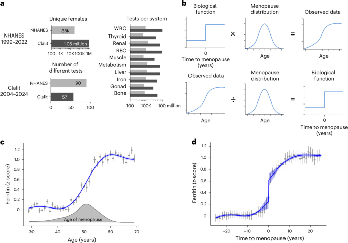
We analyzed two datasets originating from the USA (NHANES) and Israel (Clalit). NHANES is a cross-sectional health study that has been collected every 2 years from 1999 to 2022 that includes laboratory tests, health questions, exams and outcomes³⁵. Clalit is a large electronic medical record (all-comers) longitudinal dataset that includes about half the Israeli population¹⁵. We analyzed healthy laboratory test data that excluded data points with the confounding effects of medications or disease¹⁵, resulting in 1.3 million eligible female individuals aged 30–70 from years 2004–2024.

Eligibility criteria

Clalit

We analyzed all comers aged 30–70 from years 2004–2024. We excluded pregnant female individuals (N = 173,000).

NHANES

We analyzed 12 biennial waves from 1999 to 2022. We excluded pregnant female individuals (N = 1,326). For MHT comparison (Fig. 3), we only analyzed female individuals from survey years 1999 to 2019 (2022 had no MHT data owing to coronavirus disease 2019 (COVID-19)), with all covariates needed for matching: menopause status, age, poverty income ratio, smoker status, insurance status, diabetes status, ethnicity and education, with final N = 738 MHT users.

Variable definitions

Menopause status (NHANES only)

We included all nonpregnant female individuals regardless of the reason for menopause (in sensitivity analysis, we restricted to natural menopause at typical ages, showing highly concordant results with Pearson’s r = 0.97; Supplementary Fig. 7). Menopause status (female individuals only) was determined from the clinical definition of 12 months without period² together with supplemental information to confirm status. We used two questions, the first is: have you ‘had regular/at least one period in the past 12 months?’. The second follow-up question is ‘what is the reason (for no periods)?’, where we require the individual to specify ‘menopause’ as the reason. Individuals that reported having periods were defined as nonmenopausal (RHQ030/RHQ031, regular periods/at least one period in the last 12 months). Individuals were further classified as follows. Those self-reporting not having periods were classified as nonmenopausal if self-reported pregnant (this year or previous) or breastfeeding, whereas individuals who self-reported menopause were classified as menopausal (RHQ040/RHD042/RHD043, reason not having regular periods); individuals that reported any other reason for not having periods were classified as unknown (NA, not available) menopause status. RHD042 did not differentiate menopause from hysterectomy as the reason for not having regular periods but these cases were corrected afterwards as follows. We reclassified all female individuals who had a hysterectomy that reported having either a single ovary or no ovaries removed as unknown (NA) menopause age and status, because the hysterectomy would prevent them from having periods (RHQ300/RHQ305/RHQ310/RHQ320); female individuals who reported their menopause age before their hysterectomy age (RHQ291) were still included. We included participants taking oral contraceptives. Some of these individuals may not have periods, in which case, they were classified as unknown menopausal status. Finally, some individuals with indeterminate menopause status were classified according to age as follows: nonresponders to regular periods (RHQ030/RHQ031) under the age of 30 were classified as nonmenopausal, and responders over the age of 60 who reported not having regular periods were classified as menopausal (justified by the observed statistics that showed 98.3% of female individuals are nonmenopausal at age 30 and only 0.9% of female individuals were nonmenopausal at age 60). Self-reported age of menopause is top-coded at 60 in NHANES, which was extrapolated using survival modeling³⁶ as described in the ‘YoGlen method 1 for NHANES data’ section. Clalit did not have menstrual data, so menstrual status was not used for that dataset. Male individuals and the 26.8% of female individuals with unknown menopause status were imputed with a menopause age using the YoGlen algorithm described later in the methods section. We performed sensitivity analysis to consider the effects of unknown menopause status, hysterectomy and early/late menopause in Supplementary Fig. 7, which shows nearly perfect concordance of results, r = 0.97, between a restricted age range of 45–53 years with known menopause status and our reported FMP jump sizes.

MHT

NHANES

We considered female individuals as currently taking MHT if they had known postmenopause status and either (1) self-reported taking MHT or (2) reported taking any drugs containing estrogens (full list in Supplementary Table 3). For (1), we gated NHANES using RHQ540 (ever used female hormones excluding birth control): any participant reporting ‘no’ was classified as no MHT. Affirmative to any of the following was classified as yes MHT: RHQ558 (taking estrogen-only pills now; 2.9% of female individuals), RHQ566 (taking progestin-only pills now; 0.2% of female individuals), or RHQ574 (taking combination pill now; 1.1% of female individuals). After 2012, NHANES stopped asking specific questions regarding MHT usage. For (2), we used the RQQ_RX prescription drug files from each year except 2022 (not reported). We included the following types of estrogen-containing drug classes as MHT: all ‘E2’, estropipate, mestranol, all ‘estrogen’, as well as nine individuals using progesterone-only MHT.

Clalit

In Clalit, menopausal status is not recorded. We therefore defined MHT users as female individuals aged 45–55 who were prescribed at least twice the MHT drugs Angeliq (drospirenone 2 mg–estradiol hemihydrate 1 mg) or Eviana (estradiol hemihydrate 0.5 mg–norethisterone acetate 0.1 mg). We matched these individual users with controls from the same clinic, age and birth year. For each laboratory test and each group, we defined the menopause change Δ as the mean of the postmenopausal window (ages 54–60) minus the corresponding mean in the premenopausal window (ages 42–48). ΔMHT is the mean menopause change for MHT patients, and Δcontrol is the mean menopause change for the control group. MHT attenuation is defined as the relative reduction in the menopause change of MHT users compared with their matched controls: 1 − (ΔMHT/Δcontrol).

Variables and outcomes

We analyzed 90 laboratory blood tests and 31 outcomes for their time dependence with respect to inferred time of FMP. We group by systems as described in Extended Data Table 1 and Supplementary Table 2. Blood tests describe bone, liver, kidney, immune and other systems. Outcomes include signs, symptoms and diagnoses.

Preprocessing

Clalit and NHANES

All laboratory values were log-scaled and standardized to sex-specific mean and s.d. using the control reference age range of 25–45 (datasets were standardized separately). An outlier cutoff was applied at ±5 s.d. (<0.3% of data points). Log laboratory value distributions resembled normal distributions.

Clalit

Laboratory values were filtered to exclude measurements from nonhealthy individuals and from individuals taking medications that affect each specific laboratory test. To do so, we used the dataset described by Cohen et al.¹⁵, which excluded 131 chronic conditions and 5,223 drug–test pairs. Pregnancies were excluded separately. Body mass index (BMI) was linked cross-sectionally for the healthy population using the most recent measurement within the study period, and reported as median (IQR). Bootstrapping on Clalit was performed by grouping individuals by year of test date and sampling the 20 years with replacement. Test values of zero were removed (<0.3% of data points; Extended Data Table 2).

The YoGlen algorithm

We estimate the unknown age of FMP using a latent variable model³⁷ with appropriate approximations. Let p denote an arbitrary probability density function, a_m is the unknown age of FMP, m is the binary menopause status variable (available in NHANES but not Clalit), a is the known age, and y is a vector of known laboratory test values. The two results we derive are (1) how to estimate the distribution of the unknown age of FMP of each individual, $p({a}_{m}|{\bf{y}},a)$ using the observed data and (2) how to estimate mean cross-sectional laboratory trajectories as a function of the unknown time to FMP, $E[{y}_{j}{|a}]$. Jump size was estimated using resampled regression model predictions. For method 1, we used ten-repeat, tenfold cross-validation. For method 2, we used bootstrapping of $E[{y}_{j}{|a}]$.

YoGlen method 1 for NHANES data

To estimate the unknown FMP time, $p({a}_{m}|{\bf{y}},a)$ we use Bayes’ theorem $p({a}_{m}|{\bf{y}},a,m)\propto p({a}_{m}{|a},m)p({\bf{y}}|{a}_{m},a,m)$. We observed on the basis of comparison to SWAN data (Extended Data Fig. 5) that a good approximation was to use only the lowest-order term $p({a}_{m}|{\bf{y}},a,m)\approx p({a}_{m}{|a},m)$. We used draws from $p({a}_{m}{|a},m)$ to impute the unknown a_m, where p(a_m) is the reference menopause age distribution from NHANES (Fig. 1), estimated by modeling the log-hazard as a ten-knot natural spline³⁶. Female individuals with double oophorectomies (12%) were drawn separately using their own distribution. For female individuals where menopause status m is known (73.2%), conditioning on a and m restricts the permitted a_m to be before current age if nonmenopausal and after current age if menopausal. We used a discrete grid to consider all possible a_m from 20–70 at 1 year resolution. Once the $p({a}_{m}{|a},m)$ grid is estimated for each individual, we use it to draw 15 possible a_m for each individual, creating 15 completed datasets that are analyzed in parallel, and then, the results are pooled using Rubin’s rules³⁸ to account for the uncertainty in a_m.

In NHANES, most (89%) of the self-reported postmenopausal female individuals also included their age of menopause. Prior research indicates that self-reported age of menopause is accurate to about 1 year³⁹, and hence, the age of FMP for these participants was estimated assuming p(a_m) was a normally distributed true age of menopause with mean equal to their reported value and a 1-year s.d. Validation by comparison with longitudinal data from SWAN demonstrates that YoGlen fits well to the population mean for the key variables available in SWAN, FSH and E2, when only age and menstrual status are included (Extended Data Fig. 5). Inclusion of FSH and E2 into the model tended to fit worse (not shown), ostensibly because of the strong heteroscedasticity due to fluctuations in sex hormones that occurs during perimenopause^21,40 and suddenness of the transition. Therefore for NHANES the overall population trends were estimated using only menstrual status and age.

YoGlen method 2 for Clalit data

For Clalit, we did not have access to menstrual status data, precluding using YoGlen method 1, so we instead used a regression model to deconvolve each laboratory test to convert the age-dependent cross-sectional means into time-since-FMP dependent dynamics, effectively using $p({a}_{m}|{y}_{j},a,m)\propto p({a}_{m}{|a})p({y}_{j}|{a}_{m},a)$. We modeled each laboratory test as piecewise linear,

$$f\left({t|a}\right)\equiv {\beta }_{0}+{\alpha }_{0}t+\left({\beta }_{m}+{\alpha }_{m}t\right)\times I\left(t > 0\right)+\mathop{\sum }\limits_{i=1}^{p}\left({\alpha }_{i} \times(t-{t}_{i})\times I\left(t{ > t}_{i}\right)\right),$$

where $t\equiv a-{a}_{m}$ is the time to menopause, I is the indicator function (1 when true, 0 otherwise), p is the number of change points (p = 1 for Fig. 4 and p = 0 otherwise), and α_i and β_i are the regression model parameters. The β_m parameter permits a jump at FMP (t = 0). Averaging this equation over age of menopause a_m yields the cross-section mean as function of age that was fitted using least squares regression on the age-binned average values

$$\begin{array}{l}E\left[{y|a}\right]={\beta }_{0}+{\alpha }_{0}E\left[t|a\right]+{\beta }_{m}{C}_{m}\left(a\right)+{\alpha }_{m}\mathop{\displaystyle\int }\limits_{0}^{{a}}{C}_{m}\left({a}_{m}\right)d{a}_{m}\\\qquad\qquad+\mathop{\sum}\limits_{i=1}^{p}{\alpha }_{i}\mathop{\displaystyle\int}\limits_{0}^{{\max \left(0,a-{t}_{i}\right)}}{C}_{m}\left({a}_{m}\right)d{a}_{m},\end{array}$$

where $E\left[{t|a}\right]=a-E[{a}_{m}]$, E[a_m] is the average FMP age, and C_m is the cumulative density of the FMP; these values were computed numerically from a published menopause age distribution from 306,068 healthy female individuals¹⁷. For the change-point results (Fig. 4), we considered all possible t₁< 0 (premenopause) and selected the best location for the change point (t₁) on the basis of the lowest Bayesian information criterion.

Why do we call YoGlen a deconvolution, and what is the relationship to latent variable modeling?

Our latent variable is the unknown age of menopause a_m, which we seek to infer from a proxy (age, a) so that we can understand its relationship with the observed laboratory value y. This is akin to the problem of deblurring an image where $y(a-{a}_{m})$ is the true image and y(a) is the distorted image observed through the lens. We do not know the latent variable, so we have to invert what we do know, which is

$$p\left(y|a\right)={\int }_{-\infty }^{\infty }{p}_{1}\left(y,{a}_{m},a\right){p}_{2}\left({a}_{m}|a\right)d{a}_{m}.$$

In our case, y depends on the time to FMP

$$p\left(y|a\right)={\int }_{-\infty }^{\infty }{p}_{1}\left(y|a-{a}_{m}\right){p}_{2}\left({a}_{m}|a\right)d{a}_{m}={p}_{2}* {p}_{1},$$

a convolution of functions p₂ and p₁ over the latent variable, a_m. YoGlen solves the inverse problem to find p₁ (y|a−a_m) based on the observed p(y|a) and reference p₂ (a_m|a). YoGlen is thus a process of deconvolution, as it is the inverse of convolution.

Propensity score matching

Propensity score matching was used to match MHT recipients after menopause to controls both before and after menopause (1:1 matching ratio). Propensity score matches each individual to similar controls using logistic regression on a set of covariates to determine similarity²⁰. For controls, we matched to: age, poverty income ratio >1 (yes/no), smoker status (smokes now/does not), insurance status (has/does not), diabetes status (positive/negative), age of menopause, survey year ≥2005 (binary), black ethnicity (yes/no) and education ≥‘some college’ (yes/no). Black ethnicity was included as the black female cohort had higher BMD than non-black (U test P = 10⁻¹⁶, mean difference: 0.75 ± 0.02 z-score total BMD). The score balance was determined both visually using absolute mean difference and Kolmogorov–Smirnov statistic threshold of 0.1 (ref. ⁴¹). All covariates were balanced in the aftermenopause control group, but age differed in the before-menopause control. The premenopause control group differed by their median (IQR) of 51 years (48–53 years) versus 61 years (54–67 years) for the MHT group; this was expected and tolerated because the MHT users are usually postmenopausal and therefore typically older.

Regression fit lines

The regression lines in Figs. 1, 2, 4 and 5 were computed using model averages weighted by repeated cross-validation. To do so, we performed model selection (models listed below) using tenfold, ten-repeat cross-validation. We used the out-of-sample mean-squared error to choose continuous models, and area under the receiver operating characteristic curve⁴² to choose binomial models. Each fold included fitting the model to each of the FMP age estimates from YoGlen, then pooling using Rubin’s rules³⁸; pooled individual predictions were used to compute the error. In Figs. 1 and 2, we present the model average where we picked one of four Gaussian regression models at each repeat (ten-knot spline, ten-knot spline with jump, ten-knot location-scale or piecewise ten-knot location-scale) and then aggregated grid predictions from −25 to 25 years-to-FMP over the 100 total repeats. The location-scale models included joint prediction of mean and variance to mitigate issues with heteroskedasticity, probably originating from late menopause transition fluctuations²¹ (for example, Fig. 4g–i). Similarly, in Fig. 5, we present the model average where we picked one of two weighted binomial regression models at each repeat, because the outcome variables are binary and location-scale models are therefore not relevant (ten-knot spline, ten-knot spline with jump). Rare outcomes risk underfitting, and therefore, we set binomial case weights to 1 for the majority outcome and majority/minority ratio for minority outcome⁴³. In Fig. 4, we present data for female individuals with known nonmenopausal status and therefore did not require model selection. We present the ten-knot Gaussian location-scale model, which allows estimates of s.d. Best-fit lines used the mgcv package in R⁴⁴. In the analysis of MHT (Fig. 3), we used linear regression on data pooled using Rubin’s rules owing to the relatively small number of data points.

Statistics

Statistics were performed in R v4.5.1 (NHANES) and Python v3.9.23 (Clalit). All error bars/bands are standard errors. Correlations are Pearson’s. All tests are two-sided. Significance was set at P < 0.05. FDR correction used the Benjamini–Hochberg algorithm⁴⁵.

All methods are available on GitHub (https://github.com/AlonLabWIS/YoGlen).